Random Bounces Pile Up into a Bell Curve
Steel balls fall through rows of brass pins, going left or right at random at every pin. Where one lands can’t be told, yet a thousand always pile up into the same bell curve. Swap the coin for a die and the curve stays the same: that is the central limit theorem.
Scroll
The Board
Steel balls drop from the hopper on top through twelve rows of brass pins. At every pin a ball jumps left or right to the next row, and at the bottom it falls into a bin.
Where one ball will land can’t be told beforehand. After a thousand, the bins hold a curve that is high in the middle and low at the sides, and nearly the same curve every time. The gold line on the glass is that curve: twelve rows of pins, a thousand balls.
Each row has one pin more than the row above, set half a pitch across, like the five spots on a die. That arrangement is called a quincunx.
One Ball’s Path
At a pin the ball is as likely to go left as right. Twelve rows of pins are twelve coin tosses in a row.
Which bin it ends in depends only on how many times it went right: never, and it falls into bin 0 on the far left; all twelve times, and it falls into bin 12 on the far right. Right then left and left then right arrive at the same place.
In slow motion the red line is the path the ball took.
Counting Paths
A path to bin k is a choice of which k of the twelve jumps go right: C(12, k) paths in all. Each path has a chance of 1/2¹² = 1/4096. So a ball lands in bin k with probability C(12, k)/4096.
The middle bin, bin 6, has 924 paths, about 22.6%; each end bin has only one, 1/4096. The middle is high only because the most paths lead there.
This is the binomial distribution. With n rows the average bin is n/2 and the variance is n/4: for twelve rows the variance is 3, a standard deviation of about 1.73 bins. The red line on the glass is the exact distribution for the number of balls on the board now; the more balls, the closer the bins come to it.
Into a Bell
The more rows of pins, the closer the binomial distribution comes to a smooth curve, the normal curve: centred on n/2, its width growing as √n/2.
The approximation was published in 1733, and later extended to chances of going right other than one half:
C(n, k)/2ⁿ ≈ √(2/(πn)) · e^(−2(k − n/2)²/n)
The model changes to 1, 2, 4, 8 and 14 rows in turn. The more rows, the lower, wider and smoother the curve.
Swap in a Die
A coin is only the simplest nudge. Make each level’s nudge the throw of a die, moving the ball its score less 3½ bins; or move it any distance between −3 and 3 bins, all equally likely.
With one nudge the bins show the nudge’s own shape: six equal bins for the die, a flat plateau for the uniform nudge. Two nudges add up to a triangle; three are already close to a bell.
That is the central limit theorem: add up many independent nudges, each with a finite variance and none outweighing the rest, and the total is close to normal, whatever the shape of a single nudge. The figure rescales the total to one width and sets it against the normal curve; the more nudges, the smaller the gap.
Where It Shows Up
An error of measurement comes from many small, independent disturbances: temperature, vibration, the slip of a reading. Added up, such errors are often close to normal. In 1809 the normal curve was already used as the law of errors in astronomical observation.
Adult heights within one population and one sex are also close to normal, because height depends on many genes and circumstances, none of them large on its own.
Not everything is normal. Incomes, city sizes, the energy of earthquakes and daily stock-market moves have heavy tails: extremes come far more often than the normal curve says. One factor may be very large, the factors may not be independent, or they may multiply instead of add. Some distributions have no mean at all, such as the Cauchy distribution: averaging more values never settles down.
A Real Board
A real board only comes close to the ideal. Pins don’t split exactly half and half: a pin a fraction of a millimetre out of place, or a board slightly tilted, and every pin favours one side. Balls also jump more than one row at once, hit each other, and carry speed from one bounce into the next.
So a board has to stand level; the spirit level on top is there for that. Studies of the board’s dynamics find that, depending on how elastic the impacts are, the bins can stray clearly from a bell.
If every pin sends the ball right with probability p, the result is still binomial, now centred on bin np with variance np(1−p). The model shows p = 0.5, 0.65 and 0.35 in turn: the whole bell moves across and gets a little narrower.
The Bench
Let 1, 100 or 1000 balls go. Rows from 1 to 14; the chance p that a pin sends a ball right from 0.05 to 0.95; the nudge can be a die or a uniform nudge, with at most 3 levels. The histogram keeps every ball since the setting last changed; the readouts give the mean and variance, with the exact values after the slash. When a bin fills, the gate at the bottom opens and the balls fall into the drawer.
Try thisSet p to 0.7 and let 1000 balls go: which bin is the bell centred on now?
What the model leaves out
The model is larger than the original: a case about 0.85 m tall, steel balls 5 mm across, brass pins 24 mm apart. Which way a ball goes at each pin is decided by a seeded pseudorandom generator; it then falls under real gravity (9.81 m/s²) along a parabola to the next pin, with only a small rebound at each impact. The balls don’t hit each other or skip a row, so the bins follow the binomial distribution exactly, which no real board does. The die and the uniform nudge have no pins to match them: the pins sink into the board and the ball is moved once at each level. A ball beyond the edge is stopped by the case wall and falls into the end bin. A bin holds about 280 balls; when one is full the gate opens by itself.
Easy to misread
The central limit theorem is about the sum of many independent nudges being close to normal. It doesn’t say every quantity is normal, nor that data become more normal the more of it there is. Nor is the bell there because balls “prefer the middle”: every pin is even-handed, and the middle simply has the most paths leading to it. The normal curve is an approximation, in the tails above all: with twelve rows the end bin has probability 1/4096, about 0.00024, where the normal curve gives about 0.00057.
Sources
- UCL Science Collections, Quincunx, LDUGC-063 (1873, made by Tisley and Spiller to Galton’s design)
- Francis Galton (1889), Natural Inheritance, Macmillan, chapter 5, pp. 63–65, Figs. 7–9
- Francis Galton (1877), Typical Laws of Heredity, Proceedings of the Royal Institution 8: 282–301
- Abraham de Moivre (1738), The Doctrine of Chances, 2nd ed., p. 235 ff. (the paper of 12 November 1733)
- Pierre-Simon Laplace (1810), Mémoire sur les approximations des formules qui sont fonctions de très grands nombres, Œuvres complètes vol. 12
- Carl Friedrich Gauss (1809), Theoria motus corporum coelestium, book 2, section 3
- J. W. Lindeberg (1922), Eine neue Herleitung des Exponentialgesetzes in der Wahrscheinlichkeitsrechnung, Mathematische Zeitschrift 15: 211–225
- Hans Fischer (2011), A History of the Central Limit Theorem, Springer
- Francis Galton (1886), Regression Towards Mediocrity in Hereditary Stature, Journal of the Anthropological Institute 15: 246–263
- V. V. Kozlov and M. Yu. Mitrofanova (2003), Galton board, Regular and Chaotic Dynamics 8(4): 431–439
- NIST/SEMATECH e-Handbook of Statistical Methods, Cauchy Distribution
- Benoit Mandelbrot (1963), The Variation of Certain Speculative Prices, Journal of Business 36(4): 394–419
Data
The quincunx was designed by Francis Galton and made for him in London in 1873 by Tisley and Spiller (UCL Galton Collection, LDUGC-063: 360 × 290 × 52 mm, run with lead shot). He showed it at the Royal Institution in 1874, described a two-stage version in his lecture “Typical Laws of Heredity” (9 February 1877), and printed it in Natural Inheritance (1889), pp. 63–65, Figs. 7–9. Galton also coined the word “eugenics” (Inquiries into Human Faculty, 1883); the board itself is a device about chance. The normal approximation to the binomial for p = ½ is Abraham de Moivre’s, in a paper dated 12 November 1733 (translated in The Doctrine of Chances, 2nd ed., 1738). Pierre-Simon Laplace extended it to sums of many independent errors (memoir read 9 April 1810; Théorie analytique des probabilités, 1812). Carl Friedrich Gauss used the normal law for errors of observation in Theoria motus (1809). General conditions were proved by Aleksandr Lyapunov (1900–1901) and Jarl Waldemar Lindeberg (1922). The videos under Watch next are by Grant Sanderson (3Blue1Brown) and the Institute of Mathematics and its Applications. The walnut and brass board is our own model.
Watch next
The player comes from YouTube and loads only when you press play.
Follow the question
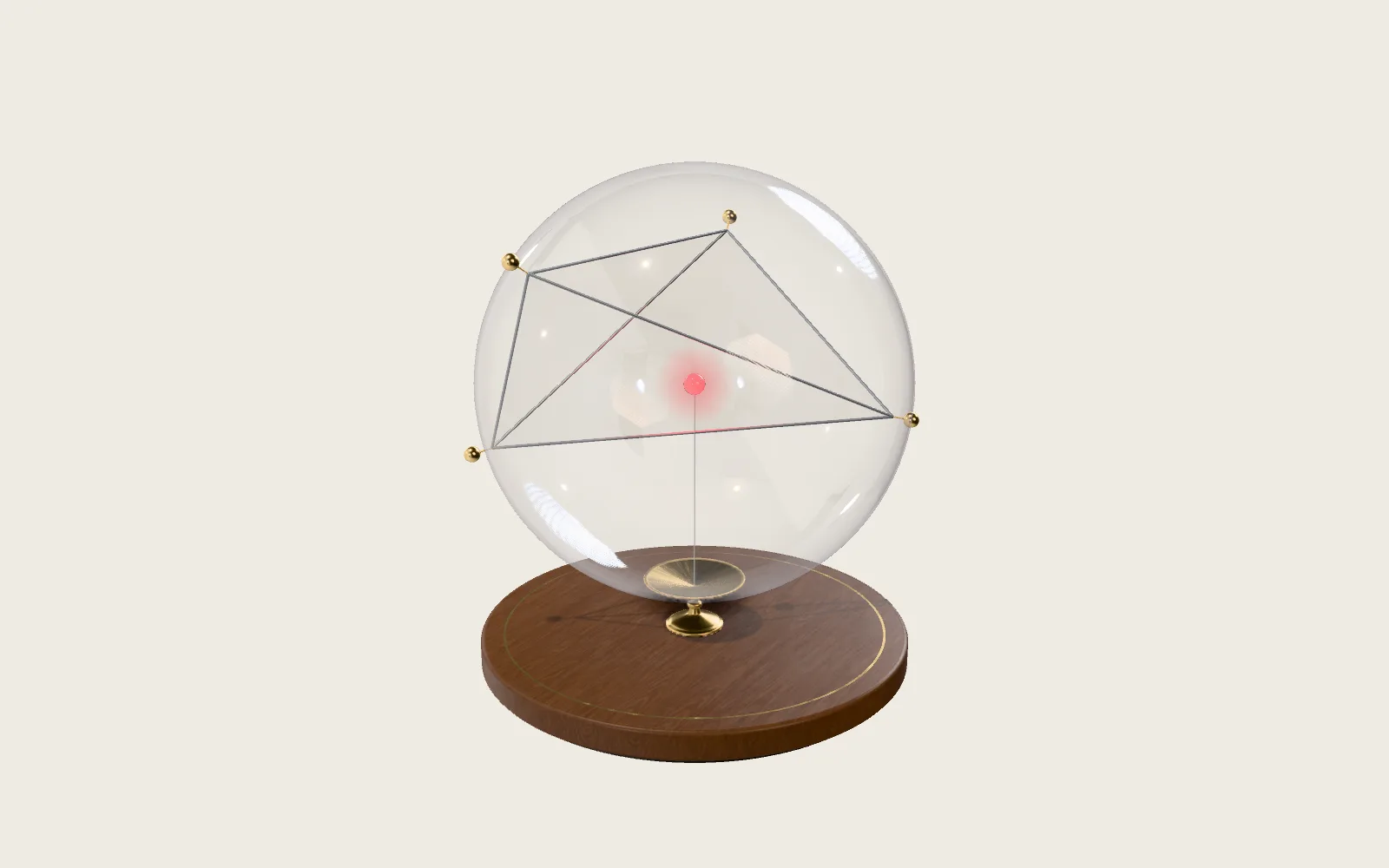 Plate M04One in Eight Random Tetrahedra Hold the CentreFour random points on a sphere make a tetrahedron that holds the centre one time in eight. Three points on a circle: one in four.
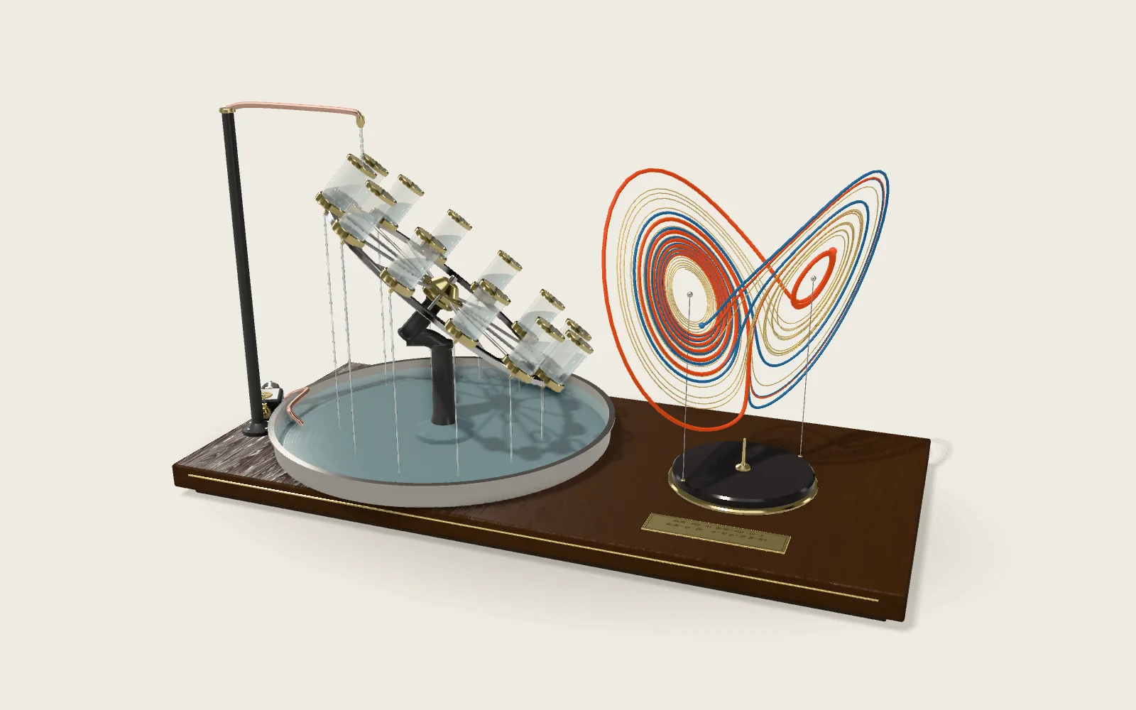 Plate M07Determined, Yet UnpredictableThree simple equations, nothing random in them. Two starts a millionth apart have nothing in common twenty time units later.