A Line That Fills a Square
Which has more points, a line segment or a square? Cantor’s answer was neither. A decade later Peano and Hilbert found something stranger: a continuous line through every point of the square. The wire in the tray is the fifth step towards it.
Scroll
As Many Points
In 1877 Georg Cantor proved that the points of a segment and the points of a square can be paired off one to one, none left over on either side. He published it the next year.
The idea is to interleave digits. Write a point of the line as t = 0.a₁a₂a₃a₄…, give the odd digits to x and the even ones to y: (0.a₁a₃…, 0.a₂a₄…). It can be read back the other way. Richard Dedekind replied that some numbers have two decimal expansions, so plain interleaving does not quite work; Cantor then corrected the proof.
In a letter to Dedekind he wrote “I see it, but I don’t believe it.” The line is often read as astonishment; the historian Fernando Gouvêa argues that Cantor was worried whether the proof had a gap.
The pairing is not continuous. Neighbours on the line, 0.4999 and 0.5000, land near the top edge and on the bottom edge of the square. In 1879 Eugen Netto proved that no map between a segment and a square is both one to one and continuous.
Through Every Point, Continuously
Give up one to one and ask only for continuity: can a line pass through every point of a square? In 1890 Giuseppe Peano gave the first example.
He split the segment into 9 pieces and the square into 3 × 3 cells, the k-th piece to the k-th cell, neighbouring pieces to neighbouring cells; then each cell into 9 again, without end. His definition is all arithmetic on base-3 digits; the paper has no picture.
The wire in the tray is the second step: 81 cells in one stroke, each step to a neighbouring cell. Curves made this way are called space-filling curves.
Hilbert’s Picture
The next year David Hilbert published a two-page note in the same journal, with a figure. He split into four each time: the segment into quarters, the square into 2 × 2, the four pieces to the four cells in turn, neighbouring pieces to cells that share a side.
Each cell is split into four again, and the curve repeats the same ∩ inside it; in the first and last cells it is turned so the ends join up. Then on, without end.
The wire of step n passes through the centres of 4ⁿ cells. At each step, the short stretch in each cell is replaced by a small ∩.
The rod in front is the segment [0, 1]. Its colours match the cells in the tray: each stretch of the line is a patch of the square.
The Limit
In a square of side 1, the wire of step n is 2ⁿ − 2⁻ⁿ long: about twice as long at each step, without bound. The Hilbert curve is none of the wires; it is their limit.
Yet the place of each t settles down. The wire of step n is nowhere farther from the limit than a cell’s diagonal, √2 / 2ⁿ, so the steps converge uniformly and the limit H(t) is continuous: change t a little, and H(t) moves only a little.
The bead sits at t = 0.3. With each step it moves a shorter way, and comes to rest near H(0.3).
Some Points, Three Times
Pick any point of the square. At each step some cell contains it; the stretches of the line for those cells nest inside each other and shrink to one t, and H(t) is that point. So no point is missed.
Some points are passed more than once. The centre of the square is a corner of four small squares, and the curve passes it three times: at t = 1/6, 1/2 and 5/6, in binary 0.0010101…, 0.1 and 0.1101010….
This is no flaw of this curve. By Netto’s theorem, any continuous curve through every point of the square must pass some points more than once.
Near Stays Near
A short stretch of the line lands in the square as a small patch. The lit cells in the tray are 64 in a row along the curve, and they always crowd into an area of about 8 × 8.
Measured on the curve of step 8: two cells whose numbers differ by k are never more than √(6k) cells apart. 6 is the exact constant for the Hilbert curve under this measure (Haverkort and van Walderveen, 2010).
The converse fails. Two cells side by side in the square can have numbers far apart: across the middle line, one lies in the first half of the curve and its neighbour in the second. Any way of putting a square in a line has places like this.
Z-Order
Interleave the binary digits of x and y and you get the Z-order number, or Morton code. G. M. Morton of IBM Canada proposed it in 1966 for a geographic database. It is Cantor’s interleaving again, in binary.
Every four cells make a Z, and four small Zs a large one. It is very fast to compute, but at the end of each block it has to jump to the next: in the right-hand tray the wire leaves the floor there and arches across. The largest jump nearly crosses the whole square.
So the limit of Z-order is not a continuous curve. The same 16 consecutive numbers are always one small patch on the Hilbert curve, and in Z-order sometimes several patches far apart; the readout gives how far apart the two farthest cells lie on each.
Its simplicity makes it common. Bing Maps interleaves the bits of a map tile’s row and column to name the tile (its quadkey).
A Family of Curves
In 1900 E. H. Moore joined four Hilbert curves end to end into a closed curve: after one round it comes back beside its start.
Peano’s curve splits into nine each time and runs as a serpentine. The same idea works with triangles, or with blocks of different sizes.
The dragon curve comes from folding paper: fold a strip in half, and in half again, then open every crease to a right angle. It does not fill a square, but four dragons from one point, each turned by 90°, run along every line of squared paper exactly once (Davis and Knuth, 1970).
Scanning Along the Curve
To turn a grey image into black and white dots, one method is error diffusion: each dot becomes black or white, and the rounding error is passed on to the next dot.
Scanning row by row pushes the error the same way every time, and stripes appear. Along the Hilbert curve the next dot is always close by and the direction keeps changing, so the error spreads more evenly (Velho and Gomes, 1991).
In the tray the bead runs along the wire through 4096 cells and settles each one black or white as it passes. This is the simplest version: the whole error goes to the next cell.
Maps and Databases
A database keeps its records in one-dimensional order. Number two-dimensional places along a space-filling curve and places near each other mostly sit near each other, so a query reads a few runs of consecutive records.
The red frame in the trays is a query. Its cells fall into a number of runs on the line; both trays show the actual count for this frame, and the Hilbert curve usually needs fewer than Z-order.
In 1994 Ibrahim Kamel and Christos Faloutsos ordered the nodes of an R-tree by Hilbert number: the Hilbert R-tree. Matrices and images are also often stored in blocks in Z-order or Hilbert order, so neighbouring elements sit closer in memory.
Cells on a Sphere
Google’s S2 geometry library numbers the Earth’s surface like this: project the sphere onto the six faces of a surrounding cube, and split each face into four along a Hilbert curve, up to 30 levels deep.
Six Hilbert curves joined end to end run once round the sphere as a closed curve; neighbouring faces run as mirror images so the ends meet. A cell’s 64-bit number is the position of its centre along that curve.
Cells at level 30 average 0.74 cm², 6 to 9 mm on a side, about 6.9 × 10¹⁸ in all. To keep the cells close in size, coordinates on the cube go through a quadratic function before they are projected onto the sphere.
The Bench
Orders 1 to 8. Drag the bead along the rod, or drag in the tray, and both move together. With “Neighbourhood” on, k cells either side of the bead light up: the Hilbert curve on the left, the same numbers in Z-order on the right.
Try thisOn the bench, raise the order from 1 to 8 with the bead at the same t. How does its place in the square change, and why do the changes keep shrinking?
What the model leaves out
Each wire in the tray is one finite step; the Hilbert curve is their limit, and no wire can be it. The wire is bent round at each corner where the mathematical polyline turns sharply. At steps 7 and 8 the cells are too small for a wire, and the curve is inlaid in the floor instead; Z-order there shows only steps between neighbours and leaves out the jumps. The Z-order wire arches over its jumps only to show them; the arches are not part of the definition. The rod stands for the parameter interval [0, 1], not for the wire’s length. The colours of the cells and the rod only match places. The first chapter’s pairing uses four decimal digits, and a point on the edge has its pin a few millimetres in from it. The dithering is the simplest error diffusion. The steel ball is engraved at S2 level 3, projected with S2’s quadratic function.
Easy to misread
A space-filling curve is not a “very dense zigzag”: every step is only an approximation; only the limit passes through every point, and some points more than once. “As many points” does not mean “continuously one to one”: Cantor’s pairing is not continuous, and a continuous one cannot be one to one. The limit of Z-order is not continuous, so Z-order is not simply a cheaper Hilbert curve. Near on the line means near in the square, but near in the square need not mean near on the line. S2 cells are not all the same size: at level 30 they range from 0.44 to 0.93 cm².
Sources
- G. Cantor (1878), Ein Beitrag zur Mannigfaltigkeitslehre, J. reine angew. Math. 84: 242–258
- F. Q. Gouvêa (2011), Was Cantor Surprised?, American Mathematical Monthly 118(3): 198–209
- E. Netto (1879), Beitrag zur Mannigfaltigkeitslehre, J. reine angew. Math. 86: 263–268
- G. Peano (1890), Sur une courbe, qui remplit toute une aire plane, Math. Ann. 36: 157–160
- D. Hilbert (1891), Über die stetige Abbildung einer Linie auf ein Flächenstück, Math. Ann. 38: 459–460
- E. H. Moore (1900), On certain crinkly curves, Trans. AMS 1: 72–90
- H. Sagan (1994), Space-Filling Curves, Springer
- H. Haverkort, F. van Walderveen (2010), Locality and bounding-box quality of two-dimensional space-filling curves, Computational Geometry 43(2): 131–147 (Hilbert WL₂ = 6, Z-order unbounded)
- G. M. Morton (1966), A computer oriented geodetic data base and a new technique in file sequencing, IBM Ltd., Ottawa
- Microsoft, Bing Maps Tile System (quadkeys interleave bits)
- C. Davis, D. E. Knuth (1970), Number representations and dragon curves, J. Recreational Mathematics 3: 66–81, 133–149 (in Knuth, Selected Papers on Fun and Games)
- L. Velho, J. de M. Gomes (1991), Digital halftoning with space filling curves, Computer Graphics 25(4): 81–90
- C. Faloutsos, S. Roseman (1989), Fractals for secondary key retrieval, PODS ’89: 247–252
- I. Kamel, C. Faloutsos (1994), Hilbert R-tree: An improved R-tree using fractals, VLDB ’94: 500–509
- B. Moon, H. V. Jagadish, C. Faloutsos, J. H. Saltz (2001), Analysis of the clustering properties of the Hilbert space-filling curve, IEEE TKDE 13(1): 124–141
- S. Chatterjee et al. (1999), Recursive array layouts and fast parallel matrix multiplication, SPAA ’99: 222–231
- S2 Geometry, S2 Cells (the S2 curve; the footnote on the centre passed three times)
- S2 Geometry, S2 Cell Statistics (cell areas by level)
- S2 Geometry Library source (Apache-2.0)
Data
Every curve on the model is computed for this page: the Hilbert curve by the quadrant-by-quadrant conversion between index and cell, Z-order by interleaving bits, Peano and Moore recursively, the dragon from the paper-folding sequence. The S2 curve on the steel ball follows the orientation tables and the quadratic projection of the S2 Geometry Library (Google, Apache License 2.0), rewritten here; cell sizes are from the S2 cell statistics page. The worst-case locality constant 6 of the Hilbert curve is from Haverkort and van Walderveen (2010); the measurements on the page are our own. The trays, wires, rod and ball are our own model.
The text, pictures and models on this page are licensed CC BY-NC 4.0: free to use and adapt for teaching and other non-commercial purposes, with credit to world.lapla.si. Third-party material listed above keeps its own licence.
Follow the question
 Plate M16More Than One ParallelReplace Euclid’s fifth postulate by “through a point off a line there is more than one parallel”, and you get a world just as consistent: triangles add up to less than 180°, and space grows exponentially.
 Plate M15A Sphere Will Not Lie FlatA sphere cannot be flattened without distortion. Every map projection gives something up: area, angles, distance or straight lines.