How Evidence Moves Belief
Balls on a table tell where another ball lies; one peg in a thousand is ill, yet most positive results are false; on a sea chart, places searched in vain send the sand to places not yet searched. Three models, each computed exactly by Bayes’ theorem.
Scroll
A Level Table
Thomas Bayes was an English Presbyterian minister who died in April 1761. His friend Richard Price found an essay among his papers and sent it with a letter to the Royal Society; it was read on 23 December 1763 and printed in volume 53 of the Philosophical Transactions as An Essay towards solving a Problem in the Doctrine of Chances.
It contains a thought experiment. On a level square table a ball W is thrown first, and it is as likely to rest on any part of the table as on any other. Through it a line os is drawn parallel to the side AD. Then a ball O is thrown p + q times, and we count how often it rests between AD and os.
The question: knowing only those counts, what is the chance that W lies between any two points we name? The table is often called a billiard table; the essay says “the square table or plane ABCD”. On the model the line is a fine brass wire, and AD is the left side.
From Counts to a Curve
Say W lies a fraction x of the table’s width from the left. Then each O lands on the left with chance x, and p on the left with q on the right has a chance proportional to xᵖ(1 − x)^q.
Before any ball, W was equally likely to be anywhere, so how much “W is at x” deserves belief is proportional to the same expression. Divided by its total area it becomes a curve of area 1, today called a Beta distribution. Bayes asked: what is the chance that W lies between two given points? The answer is the area under the curve between them.
The pin gauge behind the table draws that curve: 81 pins, each as tall as the probability density at its place, computed exactly. The brass caps span 95% of the area. The more balls, the narrower and taller the curve; the red pointer marks where W really is.
Prior Times Likelihood
In 1774 Laplace, aged 25 and without knowing Bayes’s essay, reached the same reasoning and stated it as a principle: when an event can come from several causes, the probabilities of the causes are to each other as the probabilities of the event given each cause. The causes are taken as equally likely beforehand. His Essai philosophique of 1814 states it in full: when they are not, multiply by the probability of the cause itself.
Today it is written: posterior ∝ prior × likelihood. He used it on the births in Paris from 1745 to 1770: 251,527 boys and 241,945 girls. The probability that a boy’s chance is no more than one half came out at about 1.15 × 10⁻⁴². The Beta curve of the gauge, given these numbers, gives the same.
The prior need not be flat. The blued-steel pins at the back of the gauge are a prior leaning to the left; the front row is the posterior after the same balls: it starts from the prior and is pulled by the data towards where W really is.
One in a Thousand
A disease affects 1 person in 1000. A test finds 99% of the ill as positive and clears 99% of the well as negative. Someone tests positive. How likely is it that they are ill?
The tray holds 1000 boxwood pegs, one painted red. The brass gate passing over them is the test, and a peg it calls positive rises. The red peg rises; of the 999 well pegs, about 1% rise too, about ten.
Of the 11 raised pegs, one is red: about 9%. The test is right 99% of the time, yet a positive result is true only about one time in eleven, because the well are so many: 1% of them outnumber all of the ill. In 1978, 60 physicians and students at Harvard Medical School teaching hospitals were given a similar question (one in a thousand, a false-positive rate of 5%): 27 answered 95%, and 11 gave the right answer of about 2%.
As Areas
Take numbers that are easier to see: 1 in 10 ill, a test right 9 times in 10. The tray is laid out by area: the 4 columns on the left are the 100 ill, the 36 on the right the 900 well. In each block the positives stand at the front, raised.
The left block raises 90 pegs, 10% × 90%; the right block raises 90, 90% × 10%. Of the 180 raised, exactly half are ill: 50%.
That is Bayes’ theorem as area: the prior sets how wide each block is, the likelihood how far up it is raised, and the posterior is the ill share of the raised area.
Odds and the Likelihood Ratio
In odds the theorem is one multiplication: posterior odds = prior odds × likelihood ratio. The likelihood ratio is the chance an ill person tests positive divided by the chance a well person does.
For a disease of one in a thousand the prior odds are 1 : 999. A positive result has likelihood ratio 99% ÷ 1% = 99. Multiplied, 99 : 999, about 1 : 10, the 9% from before.
A second, independent test, positive again, multiplies by 99 once more: about 9.8 : 1, or 91%. On the tray the gate passes again; the ten well pegs raised the first time each have only a 1% chance of being wrong again, and they drop. This needs the two tests’ errors to be unrelated; if one cause makes a person test wrongly both times, the second result is worth much less.
Take logarithms and the multiplications become additions. Breaking codes at Bletchley Park in the Second World War, Alan Turing measured the weight of evidence as the base-10 logarithm of the likelihood ratio, in units he called bans, and tenths of them, decibans. A positive result with likelihood ratio 99 weighs about 20 decibans.
One at a Time
Evidence can come piece by piece. Each ball that lands updates the curve: this posterior is the next prior.
Ten balls and then ten more give exactly what twenty at once give, in any order. As long as the pieces of evidence are independent, every way of splitting them arrives at the same place.
On the table the balls roll in one by one, and the gauge moves each time one comes to rest.
Different Priors, One Answer
A thinks W could be anywhere. B has made up his mind that W is probably on the right; his curve is the blued-steel row at the back. Both watch the same balls and update.
At first their curves are far apart. After a few hundred balls they nearly coincide, both close to where W really is. The more evidence, the less the prior counts.
With one exception: if someone gives a possibility a prior probability of zero, no evidence will ever change that, because zero times any likelihood is still zero.
Probability as Sand
Something lies on the sea floor. The chart is divided into squares, and the sand heaped on each is the probability that the object is there; there is one unit of sand in all.
A search of one square, if the object is there, finds it with chance d. A search that finds nothing leaves p(1 − d) in that square, and every other square is multiplied by 1 / (1 − p·d). The total stays the same; sand only flows from searched places to unsearched ones.
The brass scoop goes each time to the square where p·d is largest. When every look costs the same, this rule needs the fewest looks on average, a result of David Blackwell’s, proved by W. L. Black in 1965. When it finds nothing, the sand there sinks and everywhere else rises a little; when it finds the object, a red-headed pin goes in.
Scorpion
In May 1968 the US nuclear submarine Scorpion was lost in the Atlantic south-west of the Azores, with all 99 men aboard. The wreck lies more than 3000 metres down.
The analysts were given nine scenarios of how the loss could have happened, each with a weight for how credible it was. They simulated where the boat would have come to rest under each, and the weighted sum was a prior map: a probability for every cell.
The search ship Mizar towed cameras and sonar over the cells. Each cell searched without success was scored by how likely that search was to have found the boat there, and the map updated. The wreck was found at the end of October 1968, within 260 yards of the cell with the largest prior probability. The prior on the model is an illustrative shape: one likely track, and two other possibilities.
Air France 447
On 1 June 2009 Air France flight 447, from Rio de Janeiro to Paris, went down in the Atlantic with 228 people aboard. Within a circle of 40 nautical miles round its last known position, four searches over two years found nothing: on the surface, listening for the underwater beacons, and two by side-scan sonar.
In 2010 the French accident investigation bureau asked an American analysis firm to work it through again. The prior had three parts: 35% spread evenly over the circle, 35% a normal distribution centred on the last known position with a spread of 8 nautical miles (where past loss-of-control crashes had come down), and 30% from the drift of recovered bodies traced back. Each failed search counted as evidence: 0.77 chance of detection for the listening, 0.9 for the sonar.
If both beacons had failed, the 2009 listening could never have heard them. Without it, the probability near the last known position rose again. The 2011 search began there; about a week in, on 2 April, the wreckage showed up in sonar data, and photographs confirmed it on the 3rd: about 6.5 nautical miles north-north-east of the last known position, 3900 metres down.
The Bench
Choose a piece. The table: throw balls, change the prior, start a new table. The tray: set the base rate, sensitivity and specificity, draw a random tray. The chart: set the chance of detection and search square by square.
Try thisOn the bench tray, set the base rate to 1% and both sensitivity and specificity to 99%: how many of the raised pegs are red? Then try a base rate of 10%.
What the model leaves out
Where a ball stops across the table is uniformly random, as Bayes assumed; its depth is redrawn if it would rest on another ball, which does not change the counts. When many balls have been thrown, the oldest are collected; the counts keep them. Each pin is the exact density at its place; when the curve grows too tall the whole gauge scales down. In the chapters the tray follows the expected counts, rounded (natural frequencies); on the bench each peg is drawn at random. The chart is not a real sea. The priors and searched areas of the Scorpion and Air France chapters are simplified shapes after the published analyses, not their data; only the updating is the same. In the Air France chapter the prior weights and detection chances are the paper’s, but the searched areas are illustrative shapes, and the surface search is left out.
Easy to misread
“The test is 99% accurate” is not “a positive is 99% likely to be right”: the first is P(positive | ill), the second P(ill | positive), and the base rate stands between them. Bayes’s essay speaks of a plane, not a billiard table. A prior is not an arbitrary guess: it states what you actually believe, and different priors come together given enough data; but someone who puts a possibility at zero beforehand will never move. Two positive tests multiply by the likelihood ratio twice only if their errors are unrelated.
Sources
- T. Bayes, R. Price (1763), An Essay towards solving a Problem in the Doctrine of Chances, Philosophical Transactions of the Royal Society of London 53: 370–418
- P. S. Laplace (1774), Mémoire sur la probabilité des causes par les événements; translated with an introduction by S. M. Stigler, Statistical Science 1(3), 1986
- P. S. Laplace, Essai philosophique sur les probabilités, 1814 (the sixth principle)
- P. S. Laplace (1781), Mémoire sur les probabilités, Mémoires de l’Académie royale des sciences for 1778 (the Paris births; translated by R. J. Pulskamp)
- S. M. Stigler (2013), The true title of Bayes’s essay, Statistical Science 28(3): 283–288
- W. Casscells, A. Schoenberger, T. B. Graboys (1978), Interpretation by physicians of clinical laboratory results, New England Journal of Medicine 299: 999–1001
- A. K. Manrai et al. (2014), Medicine’s uncomfortable relationship with math, JAMA Internal Medicine 174(6): 991–993 (the 1978 question and counts)
- G. Gigerenzer, U. Hoffrage (1995), How to improve Bayesian reasoning without instruction: frequency formats, Psychological Review 102(4): 684–704
- I. J. Good (1979), A. M. Turing’s statistical work in World War II, Biometrika 66(2): 393–396
- W. L. Black (1965), Discrete sequential search, Information and Control 8(2): 159–162
- H. R. Richardson, L. D. Stone (1971), Operations analysis during the underwater search for Scorpion, Naval Research Logistics Quarterly 18(2): 141–157
- L. D. Stone, C. M. Keller, T. M. Kratzke, J. P. Strumpfer (2014), Search for the wreckage of Air France flight AF 447, Statistical Science 29(1): 69–80
- BEA, Final report on the accident on 1st June 2009 to the Airbus A330-203 F-GZCP, flight AF 447, 2012
Data
Every curve on the pin gauge is the exact Beta posterior for the balls on the table; the tray follows the expected counts (natural frequencies) unless the bench draws a random tray; the sand on the chart is updated by Bayes’s rule after every look. The chart is not a map of a real place. The search areas of the Air France chapter are simplified shapes, not the real ones; see “What the model leaves out”. The table, the tray of pegs and the chart table are our own models.
The text, pictures and models on this page are licensed CC BY-NC 4.0: free to use and adapt for teaching and other non-commercial purposes, with credit to world.lapla.si. Third-party material listed above keeps its own licence.
Watch next
The player comes from YouTube and loads only when you press play.
Follow the question
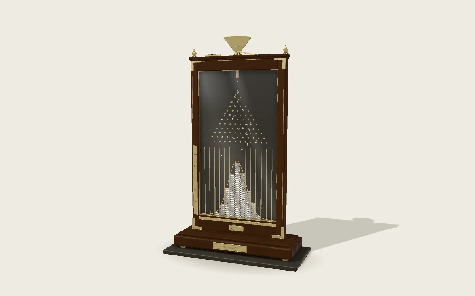 Plate M08Random Bounces Pile Up into a Bell CurveOn a Galton board each steel ball goes left or right at random at every pin. After a thousand balls, the bins always show the same bell curve.
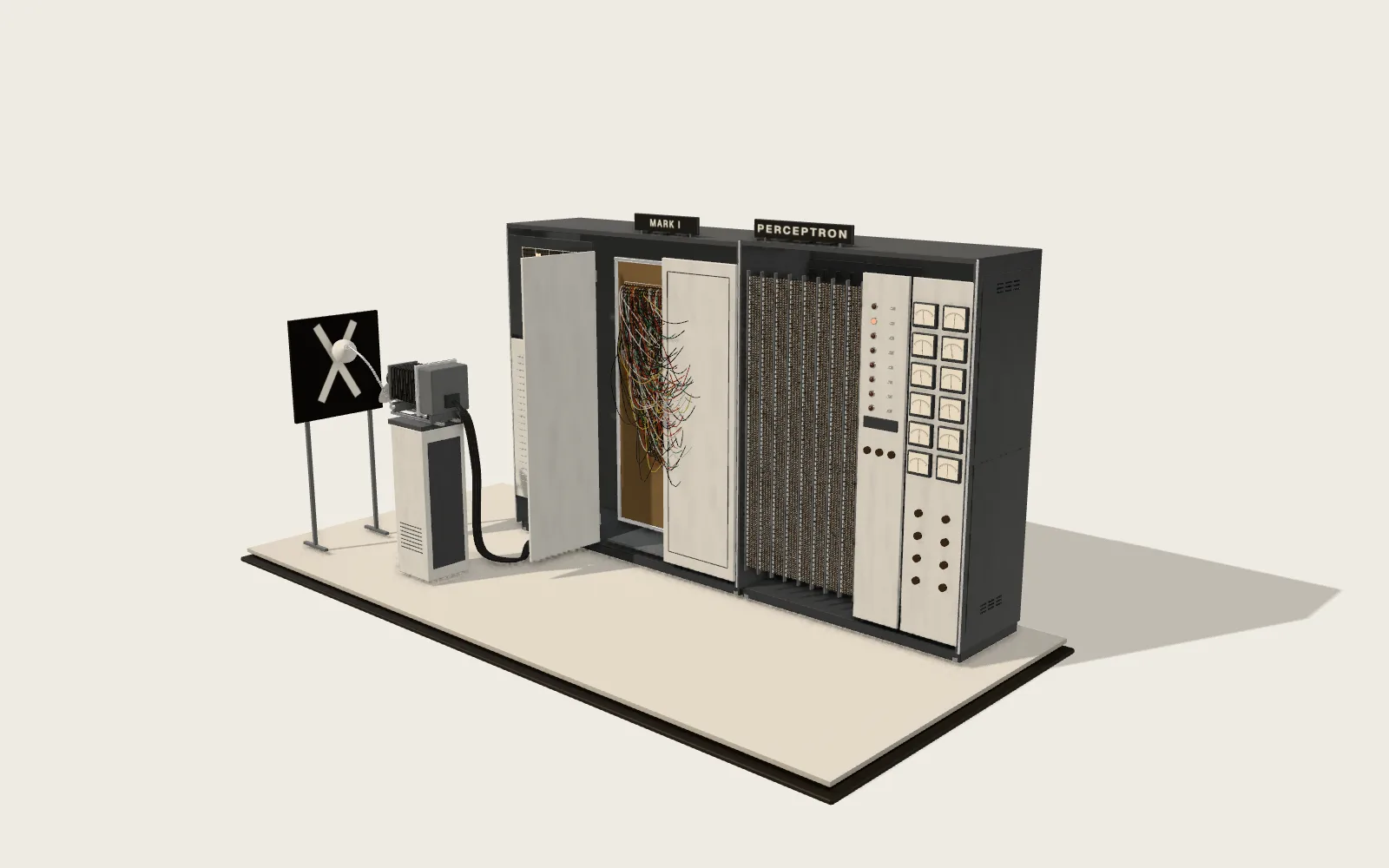 Plate C15The Mark I PerceptronA machine that learned letters from examples: four hundred photocells to see, 512 randomly wired units in between, and motor-driven potentiometers to remember.