The Event Horizon Telescope
Not one telescope but eight, at six places on Earth. In April 2017 they watched one black hole at once, each timed by an atomic clock, to resolve as finely as an Earth-sized dish.
Scroll
An Earth-Sized Telescope
How fine a detail a telescope can resolve depends on its wavelength divided by its width. The Event Horizon Telescope observes at a wavelength of 1.3 mm. In 2017, seen from the direction of M87*, the two telescopes furthest apart in the array were about 10,700 km apart.
1.3 mm divided by 10,700 km is about 25 microarcseconds. The papers give an effective resolution in the images of about 20 µas; the official comparison is reading a newspaper in New York from a café in Paris. The ring round M87* is 42 µas across. Why there is a ring at all is told in the plate “Where Not Even Light Escapes”.
1.3 mm ÷ 10,700 km ≈ 25 µas · images about 20 µas · ring 42 µas
Two Dishes, One Set of Stripes
The same wavefront reaches two telescopes at different moments. Line up the two recordings, multiply them and average, and out comes one complex number: how well a pattern of light and dark stripes on the sky matches the brightness round the black hole, and how far the stripes must shift to match it best.
The stripes’ spacing is the wavelength divided by the distance between the two telescopes, as seen from the source; they run at right angles to the line between them. One pair of telescopes measures one set of stripes, not a picture. Mark each set as a point, further from the centre for finer stripes: this map is called the u-v plane.
Stripe spacing = wavelength ÷ projected baseline · one pair = one point on the u-v plane (and its mirror)
The Earth Turns
The Earth turns. Seen from M87*, the line between two telescopes turns with it and changes length, so a pair draws an arc across the u-v plane. On the night of 11 April 2017, the seven telescopes that could see M87*, taken in pairs, drew these arcs. The telescope at the South Pole cannot see M87*.
The more arcs, the more of the stripes are measured, and the closer the rebuilt picture comes to the sky. The picture here is computed in the browser: a ring of known size stands in for the truth on the sky; only the cells the arcs pass through are kept, and a picture is rebuilt from them.
Seven telescopes see M87* · 21 pairs (two of them at one site, too short) · this page’s ring model, not real data
Filling the Gaps
A whole night still measures only a few thin arcs across the u-v plane, and most of it stays empty. Turned straight back into a picture, the measured part gives one full of stripy artefacts (left).
Countless pictures fit the data. An imaging algorithm picks the most reasonable one: no brightness below zero, no needless flicker between neighbouring spots, as plain as possible where nothing was measured. This page uses a small version of such a “regularised maximum likelihood” method (right).
Left: the measured cells transformed straight back · right: rebuilt by regularised maximum likelihood
Cut Open: One Station
This is APEX on the Chajnantor plateau in Chile, about 5,100 m up, one of the EHT’s eight telescopes in 2017. It was made from an ALMA prototype antenna; its main reflector is 12 m across with a focal length of 4.8 m, and the whole antenna weighs about 125 tonnes.
Radio waves strike the main reflector and head for its focus; on the way, a 0.75 m subreflector folds them back through a hole in the middle of the dish into the Cassegrain cabin, and mirrors send them along the elevation axis into a Nasmyth cabin at the side. The 1.3 mm receiver used for the EHT sits there.
Main reflector 12 m · focal length 4.8 m · subreflector 0.75 m · two Nasmyth cabins · about 125 tonnes
264 Panels
The main reflector is made of 264 aluminium panels in 8 rings, on a carbon-fibre backup structure of 24 sandwich segments. Adjusters behind each panel push it to its place on the paraboloid.
In 2017 the surface was accurate to about 17 µm (rms). By Ruze’s formula, that leaves 1.3 mm waves about 97 % of their efficiency; a 100 µm error would leave about 40 %. Early in 2018 the panels and subreflector were replaced, bringing the error to about 10 µm.
264 panels · 8 rings · 17 µm (2017) → 10 µm (2018) · efficiency = e^−(4πσ/λ)²
Bringing 230 GHz Down
A 1.3 mm wave swings about 230 billion times a second, far too fast to record. The receiver mixes it with a local signal at 221.1 GHz, which brings 226.1 to 230.1 GHz down to 5 to 9 GHz. The mixers are superconducting (SIS) and must be kept at a few kelvin.
APEX’s receiver is PI230, built by the Max Planck Institute for Radio Astronomy and installed in a Nasmyth cabin in 2015. The lowered signal is digitised at 2 bits: two bands 2 GHz wide, two polarisations, about 32 billion bits a second in all.
Local signal 221.1 GHz · 226.1–230.1 GHz → 5–9 GHz · 2 bits · 32 Gbit/s
A Clock at Every Station
No cable joins the telescopes. Every station has a hydrogen maser, an atomic clock that sets the receiver’s local signal and the time stamps on the data. APEX’s maser was installed in 2010, in a cabinet held to ±0.1 °C beside a container; its signal runs to the antenna on cables 85 m long.
The goal is a frequency that drifts by no more than 1.5 parts in 10¹⁴ over 10 seconds. At that, even at 0.87 mm, the signal keeps nearly all its coherence through an integration. GPS lines the stations’ clocks up to within tens of nanoseconds; what is left is solved for at the correlator.
σ(10 s) = 1.5 × 10⁻¹⁴ · GPS timing to tens of nanoseconds
Data by Air
Each station records 32 billion bits a second. In April 2017 the array recorded about 350 terabytes a day, about 3.5 petabytes of raw data in all (the EHT’s figure; its scientists have also written about 4 PB). Sending that over the internet would take too long, so it went onto helium-filled hard disks, flown to the correlators.
One recorder writes 16 billion bits a second, sliced in time across 32 disks in four removable modules. APEX’s recorders sit in a control container about 50 m from the antenna. With no flights to the South Pole from February to October, the disks from there reached MIT’s Haystack Observatory only on 13 December 2017.
32 Gbit/s · about 350 TB a day · about 3.5 PB · South Pole disks arrived 13 December
Line Up, Multiply
A wavefront reaches the stations at different times, up to tens of milliseconds apart. The correlator lines the recordings up with a model of the Earth’s geometry and each station’s clock, multiplies them in pairs and averages, giving one complex number every 0.4 s. In 2017 the work was split: MIT Haystack took the band at 227.1 GHz and the Max Planck Institute for Radio Astronomy in Bonn the band at 229.1 GHz, each on more than a thousand processor cores running the DiFX software.
The air above each station makes the phases jump. But add up the three phases between three telescopes, round the triangle, and each station’s error comes in once with a plus and once with a minus and cancels. That sum, the closure phase, depends only on the sky.
Closure phase = φ₁₂ + φ₂₃ + φ₃₁ · station errors cancel
Four Teams, Working Blind
Four teams took the same data from 11 April and imaged it for seven weeks without talking to one another: two with CLEAN, two with regularised maximum likelihood. All four got a ring, brighter in the south.
Then three pipelines (DIFMAP, eht-imaging, SMILI) each surveyed a thousand to tens of thousands of combinations of settings, keeping those that recovered known test pictures. Here, this page’s one set of simulated data rebuilt with three settings: the details differ, the ring is in each.
Four teams · seven weeks · three pipelines · about 49,000 parameter sets
Two Black Holes
M87*: shown on 10 April 2019, a ring 42 ± 3 µas across round a black hole of about 6.5 billion solar masses, 55 million light years away. The picture comes from one night, 11 April 2017; the other nights, imaged on their own, agree. In 2021 its polarised image showed the direction of the magnetic field round the ring.
Sagittarius A*, at the centre of our galaxy: shown on 12 May 2022, a ring 51.8 ± 2.3 µas across, about 4 million solar masses, some 27,000 light years away. Gas goes round it in minutes, so the ring changes within a night, which made it much harder to image. The South Pole telescope can see it. Telescopes in Greenland, at Kitt Peak and NOEMA have joined since; in test observations at 0.87 mm the finest stripes reached 19 µas.
M87* 42 µas (2019) · Sgr A* 51.8 µas (2022) · 0.87 mm: 19 µas
Taken Apart
The subreflector on its four legs, the 264 panels, the backup structure, the Cassegrain cabin, the two Nasmyth cabins, the yoke and the pedestal come apart, layer by layer.
Whichever part the pointer rests on is lifted out and the rest fade; left alone, the parts are all named.
Build an Array
The globe holds the eight telescopes of 2017. The lever is how far the Earth has turned; every pair that can see the black hole draws its own arc on the u-v plane, and the picture beside it is rebuilt as they go.
The switches are the six sites; the choice is the black hole. The South Pole telescope cannot see M87*, but it can see Sagittarius A*.
Try thisWith only the telescopes in Chile and Hawaii, after a whole night of turning, can the ring still be seen in the rebuilt picture? And with Spain added?
What the model leaves out
The antenna follows APEX’s published figures: a 12 m main reflector of 264 panels in 8 rings, a 4.8 m focal length, a 0.75 m subreflector, two Nasmyth cabins; the backup structure, the cabins’ insides, the yoke and the pedestal are shown in outline, not from drawings. The control container really stands about 50 m away; here it is moved close. The telescopes on the globe are drawn many times larger than life. The u-v tracks use the stations’ positions from the papers and the source’s position, assume a telescope can observe whenever the source is 10° above its horizon, and set the stripes at 228.1 GHz; real observing has each station’s own limits (M87* was dropped below 20° at ALMA), weather and faults. The “truth” in the rebuilt pictures is a ring this page sets up (its size and bright side as for M87*), not real data; the visibilities are taken straight on the grid’s cells, with no noise and no atmosphere. Real imaging has to deal with noise and calibration errors, and leans on quantities such as closure phases that station errors don’t touch.
Some common misreadings
The picture is not a photograph taken with one press of a shutter. The data were recorded through a whole night, the Earth’s turning swept the baselines across the u-v plane, and an algorithm rebuilt the picture; its colours are added and stand for radio brightness. Nor is the Event Horizon Telescope a dish the size of the Earth: it resolves as finely as one would, but the signal it gathers comes only from its telescopes’ own areas, and it measures only part of the u-v plane. And the dark patch in the middle is not the black hole itself but its shadow, magnified by bent light: see the plate “Where Not Even Light Escapes”.
Common questions · 3
- How fine a detail can the Event Horizon Telescope resolve?
1.3 mm divided by 10,700 km is about 25 microarcseconds. The papers give an effective resolution in the images of about 20 µas; the official comparison is reading a newspaper in New York from a café in Paris.
01An Earth-Sized Telescope ↑- Why were the data flown on hard disks instead of sent online?
Sending that over the internet would take too long, so it went onto helium-filled hard disks, flown to the correlators.
09Data by Air ↑- What is a closure phase?
The air above each station makes the phases jump. But add up the three phases between three telescopes, round the triangle, and each station’s error comes in once with a plus and once with a minus and cancels. That sum, the closure phase, depends only on the sky.
10Line Up, Multiply ↑
Sources
- EHT Collaboration (2019): M87* Paper I, ApJL 875, L1 (eight stations, six sites; baselines 160 m to 10,700 km; about 25 µas; the 11 April image; ring 42 ± 3 µas; mass 6.5 × 10⁹; 16.8 Mpc)
- EHT Collaboration (2019): Paper II, the array and instrumentation, ApJL 875, L2 (station positions; maser σ(10 s) = 1.5 × 10⁻¹⁴; recorders at 16 Gbit/s, 32 disks, four modules; local signal 221.1 GHz; APEX surface 17 → 10 µm; recorders in a container about 50 m away)
- EHT Collaboration (2019): Paper III, data processing and calibration, ApJL 875, L3 (the 227.1 / 229.1 GHz bands correlated at Haystack and Bonn; DiFX; closure phases; ALMA stopping below 20°)
- EHT Collaboration (2019): Paper IV, imaging, ApJL 875, L4 (four teams, seven weeks, CLEAN and RML; the DIFMAP, eht-imaging and SMILI parameter surveys)
- EHT Collaboration (2019): Paper VI, the shadow and mass of the central black hole, ApJL 875, L6
- EHT Collaboration (2021): Paper VII, polarisation, ApJL 910, L12 (APEX’s 2017 receiver in a Nasmyth cabin)
- EHT Collaboration (2022): Sgr A* Paper I, ApJL 930, L12 (ring 51.8 ± 2.3 µas; about 4 × 10⁶ solar masses; variability within an hour)
- EHT Collaboration (2022): Sgr A* Paper III, imaging, ApJL 930, L14
- Event Horizon Telescope press release (10 April 2019): 20 µas, a newspaper in New York read from a café in Paris; hydrogen masers; about 350 TB a day
- Event Horizon Telescope: FAQ (about 3.5 PB of raw data in 2017; about 8 hours a night; not a classical photograph)
- Event Horizon Telescope blog (15 December 2017): the South Pole disks reached Haystack on 13 December
- C. Goddi et al. (2019): First M87 Event Horizon Telescope Results and the Role of ALMA, ESO Messenger 177 (about 4 PB; helium-filled disks; data shipped)
- ESO eso1907: the first image of a black hole
- ESO eso2105: M87* in polarised light (2021)
- ESO eso2208: the first image of the black hole at the centre of the Milky Way (2022; about 27,000 light years; gas orbits in minutes)
- ESO eso2406: Sgr A* in polarised light (2024)
- A. W. Raymond et al. (2024): test observations at 345 GHz, AJ 168, 130 (19 µas)
- R. Güsten et al. (2006): The Atacama Pathfinder EXperiment (APEX), A&A 454, L13 (a modified ALMA prototype with two Nasmyth cabins; 264 aluminium panels in 8 rings on 24 CFRP sandwich segments; f = 4.8 m; 0.75 m subreflector; about 125 tonnes)
- APEX: the telescope (264 panels, 0.75 m subreflector, two Nasmyth cabins and a Cassegrain cabin)
- ESO: APEX’s PI230 receiver (built by MPIfR, installed in a Nasmyth cabin in 2015, dual polarisation, sideband-separating)
- A. Roy et al. (2012): VLBI equipment at APEX (the maser installed in 2010, a cabinet held to ±0.1 °C)
- ALMA Technical Handbook (Cycle 12): 12 m antennas, the 4 K closed-cycle cryostat
- J. Ruze (1966): Antenna tolerance theory — a review, Proc. IEEE 54, 633
- A. R. Thompson, J. M. Moran, G. W. Swenson (2017): Interferometry and Synthesis in Radio Astronomy (u-v coordinates, Earth-rotation synthesis)
- NASA: Earth fact sheet (mean radius 6,371 km)
Data
Station positions from EHT Collaboration Paper II (ApJL 875 L2, 2019), Table 2; source positions from SIMBAD. The u-v tracks, the ring model and the pictures rebuilt from it are computed by this page; they are not EHT data. The antenna follows the published layout of APEX (Güsten et al. 2006; apex-telescope.org); the model, the imaging code and the words are the site’s own. No EHT, ESO or MPIfR endorsement is implied. The globe’s map uses the same elevation grid as the site’s other globes. Material presets, parts and the softbox studio of the site’s model kit are ported from AirsupHQ/machine-skill (MIT, © 2026 Air Supply Technologies Inc.).
The text, pictures and models on this page are licensed CC BY-NC 4.0: free to use and adapt for teaching and other non-commercial purposes, with credit to world.lapla.si. Third-party material listed above keeps its own licence.
Cite this plate
Laplace’s Mini World, Plate F21, “The Event Horizon Telescope”, https://world.lapla.si/en/eht/, CC BY-NC 4.0, updated 2026-10-19.
Follow the question
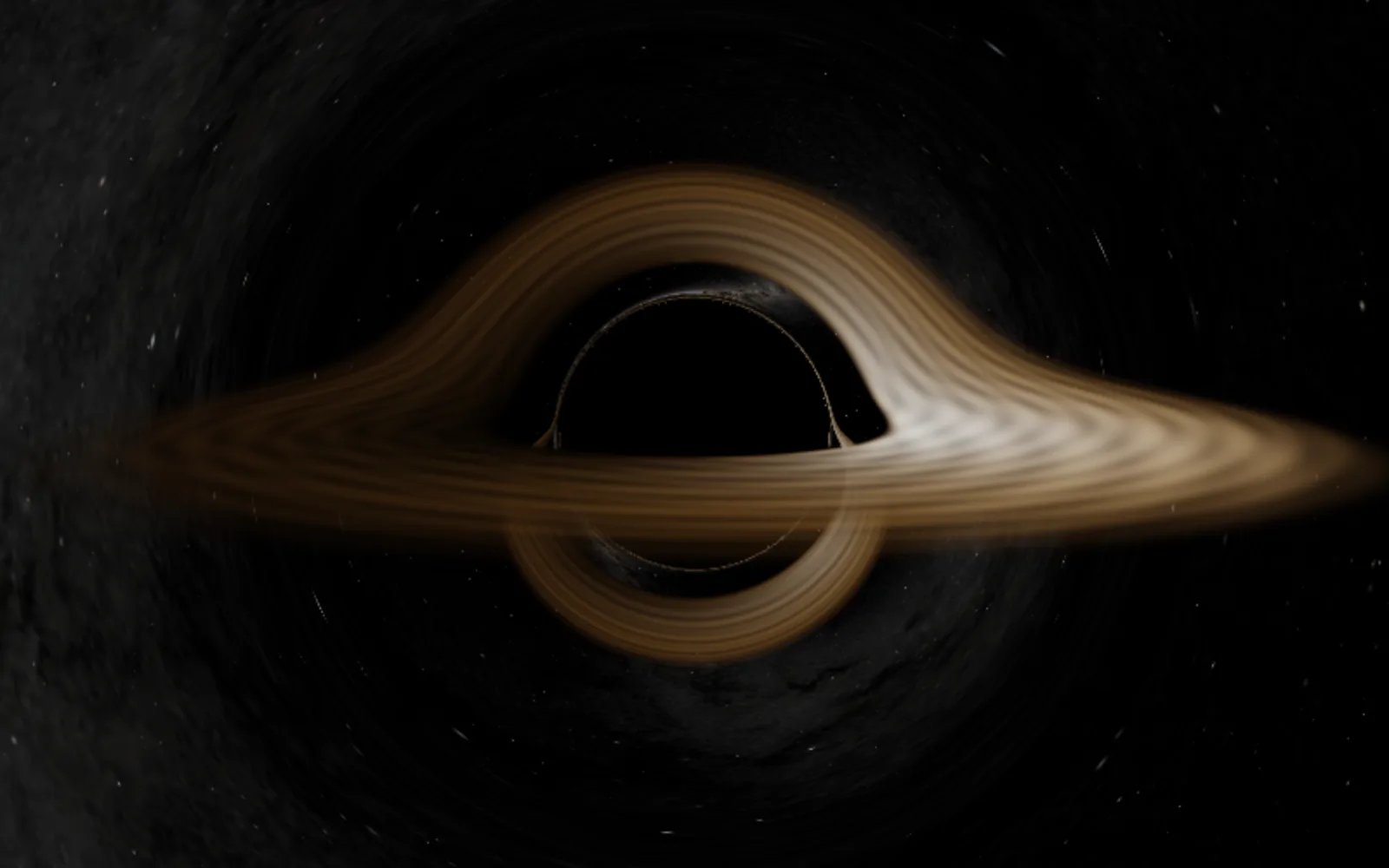 Plate 38Where Not Even Light EscapesA black hole packs so much matter into so small a space that not even light can get out. It is dark itself, but the light it bends around it draws a bright ring.
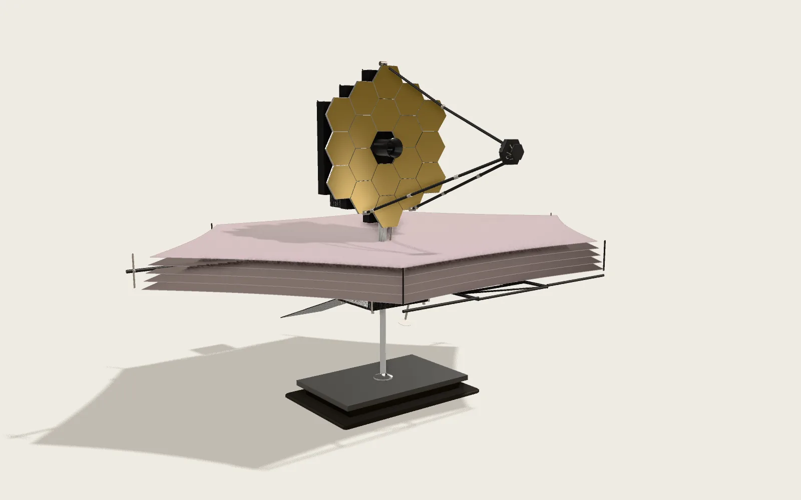 Plate F09The Webb Space TelescopeEighteen gold-coated segments make one 6.5 m mirror, and five layers of film keep the Sun’s heat off it. It was launched folded and unfolded itself in space over two weeks.