Tracing a Model’s Steps
Asked for the capital of the state containing Dallas, a model says Austin. An attribution graph finds a step via Texas, in a stand-in model, and only in part.
Scroll
Between Dallas and Austin
Give the language model Claude 3.5 Haiku “Fact: the capital of the state containing Dallas is” and it goes on with Austin, at 98%. Getting it right seems to take two steps: Dallas is in Texas; the capital of Texas is Austin.
Does it really take those two steps inside? It might instead have seen a similar sentence in its training text and remembered the answer. From outside, both ways write Austin.
On the stand is a manual telephone switchboard: on the left a row for each word of the prompt, on the right the words the model might write next, Austin lit. The panel in the middle is what we want to see.
Prompt: Fact: the capital of the state containing Dallas is · next word: Austin, 98%
Parts You Can Read
Most of a model’s neurons do many jobs: one responds to many unrelated things, which makes them hard to read. So the researchers first train a “cross-layer transcoder”: layers of “features”, each reading from one layer of the model and writing into the MLP outputs of that layer and every later one, trained to rebuild the MLPs’ outputs with as few features active at once as possible. For what a feature is, see “Sparse Autoencoders”.
Put these features in place of the model’s MLPs and you have a replacement model. The set made for Claude 3.5 Haiku has 30 million features. It is not the model: on a small 18-layer model, the largest set picks the same next token as the model about half the time (on tokens the model got right, but with less than 80% confidence).
So for one sentence they build a local replacement model: the attention patterns are copied from the real model on that sentence, and wherever a layer falls short an “error node” makes up the difference. On that sentence every number then matches the model’s; the authors add that this does not guarantee the two use the same mechanisms. The top-left row of the feature panel, marked error, is an error node: no cord leads into it.
Features: read from one layer, write to the later ones · Haiku’s set: 30 million features · 18-layer model: the same token about half the time · error nodes: the difference
Effects Drawn as Wires
On that sentence they draw an attribution graph. It has four kinds of node: the prompt’s tokens, the features active at each position, error nodes, and candidate next tokens (enough for 95% of the probability, up to 10). An edge is one node’s direct effect on another, the first one’s activation times a weight; a feature’s input is the sum of the edges into it.
Such a graph starts with millions of edges. Only the most important are kept: with the default settings about a tenth of the nodes stay, and about a fifth less of the behaviour is explained; what remains often still has hundreds of nodes and tens of thousands of edges. The researchers then group features with similar meanings by hand into “supernodes” and give each a rough name, such as Texas or “say a capital”.
The middle panel on the stand holds only 6 supernodes: a lamp is a group, a patch cord an edge, thicker for a stronger effect (this page’s drawing, in three steps); the thin dark ones stand for some of those pruned.
Nodes: tokens · features · errors · candidates · edges: activation × weight · pruning: about a tenth of the nodes, a fifth less explained · supernodes: grouped by hand
Through Texas
In the graph, Dallas features (with a little from state features) turn on a group of features about Texas; the word capital turns on features that “say a capital”. Texas and “say a capital” together push Austin up, directly and through a group of “say Austin” features.
There is also a shortcut, from Dallas straight to “say Austin”. The two steps and the shortcut are there at once. The paper says the replacement model really does reason in several steps here, and warns that the graph simplifies the true mechanism a great deal.
On the stand, the lit red cords are the two-step path: Dallas → Texas → say Austin → Austin, the rest dimmed; the dark red ones are the capital path; the thin black ones include the shortcut.
Dallas → Texas → say Austin → Austin · capital → say a capital → Austin · shortcut: Dallas → say Austin
Turning Texas Down
A graph is a hypothesis. The evidence is found back in the real model: hold a group of features at a negative multiple of their activation, or add another group in, and see whether later features and the answer change as the graph predicts. On the stand, a thrown key marks an intervention and a red lamp the group held down.
Hold the Texas group at −2× and the “say Austin” features fall to 21% of their activation; Austin falls from 98% to 6%. Hold “say a capital” at −2× and the model says Texas instead (76%).
Hold Texas down and add California features, found in “the capital of the state containing Oakland”, at +2×: the answer becomes Sacramento (97%); Georgia gives Atlanta (78%). British Columbia, China and the Byzantine Empire need +8×, and give Victoria, Beijing and Constantinople.
Texas −2×: Austin 98% → 6% · say a capital −2×: Texas 76% · Texas −2×, California +2×: Sacramento 97%
The Rhyme Comes First
Ask the model for a rhyming couplet: “A rhyming couplet: / He saw a carrot and had to grab it,”. It goes on: “His hunger was like a starving rabbit”.
A language model writes one token at a time, so it could find its rhyme as it goes. Yet on the line break, before the second line starts, features for rabbit and habit are already at work, drawn out by features for rhyming with “it”; they push the line to end in rabbit. The authors call this planning, meaning exactly these measured effects.
Change them and the ending changes. On the last word alone: rabbit 81%, habit 19%; hold rabbit at −10× and habit rises to 95%. Hold rabbit and habit down and inject green on the line break, rewrite the whole line 500 times, and 73% end in green, as in “freeing it from the garden’s green”. The intervention works only on the line break. Injecting rabbit or green into 25 randomly chosen poems changed the ending to the injected word in 70% of cases; features for a planned word were found in only about half of the poems.
On the line break: rabbit, habit · rabbit −10×: habit 95% · green injected: 73% of lines end in green · 25 poems: 70%
What It Says, What It Does
Ask 36 + 59 and the model says 95. In the graph it works two ways at once: one path only estimates size, “about 36 plus about 60”, giving “the sum is near 92”; another only minds the last digit, “ends in 6 plus ends in 9”, and looks up “the sum ends in 5”. Together they give 95. The last-digit step looks like a learned table of one-digit sums.
Hold down “ends in 6” and it answers 98: the tens stay, the last digit becomes that of 9 plus 9. Hold down “ends in 9” and it answers 91, not 92; the authors say such numerology must be taken with a grain of salt.
Ask how it got the answer and it says: I added the ones (6 + 9 = 15), carried the 1, then added the tens (3 + 5 + 1 = 9). The graph has no such carry. The paper’s reading: the model learns to explain by imitating explanations in its training text, and learns to do the sum by another process; it has no “metacognitive” insight into this skill. That is the result for this one sum.
Size: ~36 + ~60 → sum near 92 · last digit: _6 + _9 → ends in 5 · together: 95 · its own account: carry the 1
What It Cannot See
The authors say their attribution graphs give a satisfying explanation for about a quarter of the prompts they have tried; the examples in the paper are the successes, and even these show only a small part of the model’s mechanisms.
The graph traces the replacement model, not the model itself, so what it says about the model is a hypothesis to test with interventions. It does not explain why attention looks where it does; error nodes come from nowhere and cannot be read; it shows only active features, not why others stay dark; it has not been used on prompts longer than about a hundred tokens. Even for a prompt of a few dozen words, reading a graph takes a few hours.
The transcoders cost compute too: the authors estimate about 210 H100 hours to train 2 million features for the open model Gemma 2 2B. In May 2025 the tools for drawing attribution graphs were released openly, for open models such as Gemma-2-2B and Llama-3.2-1B. For what grows inside a network as it learns a rule, see “Learning by Heart, Then Learning the Rule”.
About a quarter of prompts: a satisfying explanation · it traces a replacement model · why attention looks where it does: unseen · reading a graph: hours
Taken Apart
On the stand: a wooden cabinet holding three jack panels, the prompt’s words on the left, features in the middle, the next word on the right; each panel of hard-rubber jack strips, brass jacks, lamps and typed name strips; patch cords with a plug at each end; and in front the key shelf, with spare plugs, supervisory lamps and lever keys. The switchboard is a metaphor: a real one connects one line at a time, while an attribution graph holds many connections acting at once, strong and weak, positive and negative.
Cabinet · prompt panel · feature panel · next-word panel · patch cords · key shelf
The Bench
This is a toy network written for this page, not Claude: a few named units with weights set by hand. Pick a city, switch off the state feature or “say a capital”, or swap the state for another, and watch the answer and the cords change.
A cord’s thickness is the toy’s activation × weight; switching a unit off holds its activation at 0.
A toy network · weights set by hand · not Claude
Try thisIn the lab, switch off “say a capital”: what does the toy say instead? And with the state feature off too?
What the model leaves out
The switchboard is this page’s model. Its panels carry only the few supernodes of the papers’ simplified graphs; a real graph has hundreds of nodes, tens of thousands of edges and error nodes. Cord thickness and lamp brightness come in three steps, a drawing, not measured values; the percentages in the HUD are the papers’ own. Edges in an attribution graph can be positive or negative; only positive ones are drawn. The addition chapter folds the graph’s layers into two. The network on the bench is a toy.
A common misreading
An attribution graph is not the model’s wiring: it traces a replacement model’s computation on one sentence, its edge weights do not exist in the model itself, and its claims are tested with interventions. “Reasoning” and “planning” are the authors’ names for measured effects (turn a group of features down or in, and the answer follows), not a claim that the model thinks as people do. The two-step path and a shortcut are both in the graph, so it does not show the model remembered nothing. Keep the fractions apart: about a quarter of prompts explained to the authors’ satisfaction; about half the time the same token as the model, for the replacement on the 18-layer model; planned-word features in about half the poems; injections working in 70% of 25 poems. The model’s account of its sum differs from the graph; the paper does not say it lies.
Common questions · 5
- What happens inside a model on its way to “Austin”?
In the graph, Dallas features (with a little from state features) turn on a group of features about Texas; the word capital turns on features that “say a capital”.
04Through Texas ↑- How is an attribution graph drawn?
On that sentence they draw an attribution graph. It has four kinds of node: the prompt’s tokens, the features active at each position, error nodes, and candidate next tokens (enough for 95% of the probability, up to 10).
03Effects Drawn as Wires ↑- How is an attribution graph tested?
A graph is a hypothesis. The evidence is found back in the real model: hold a group of features at a negative multiple of their activation, or add another group in, and see whether later features and the answer change as the graph predicts.
05Turning Texas Down ↑- Does a language model plan a rhyme ahead?
A language model writes one token at a time, so it could find its rhyme as it goes. Yet on the line break, before the second line starts, features for rabbit and habit are already at work, drawn out by features for rhyming with “it”; they push the line to end in rabbit.
06The Rhyme Comes First ↑- How much do attribution graphs explain?
The authors say their attribution graphs give a satisfying explanation for about a quarter of the prompts they have tried; the examples in the paper are the successes, and even these show only a small part of the model’s mechanisms.
08What It Cannot See ↑
Sources
- E. Ameisen et al. (2025): Circuit Tracing: Revealing Computational Graphs in Language Models, Transformer Circuits Thread (cross-layer transcoders, the replacement model, attribution graphs, pruning, interventions; the limitations)
- J. Lindsey et al. (2025): On the Biology of a Large Language Model, Transformer Circuits Thread (examples in Claude 3.5 Haiku: two-step reasoning, planning a rhyme, addition; how much it explains)
- Anthropic (2025): Tracing the thoughts of a large language model (a summary of both papers)
- Anthropic (2025): Open-sourcing circuit tracing tools (the open library and the Neuronpedia front end)
- circuit-tracer (GitHub, MIT licence): a library for attribution graphs on open models
- S. G. McMeen and K. B. Miller (1912): Telephony (a manual switchboard’s jacks, plugs, cords and key shelf; for the set)
Data
Attribution graphs, the replacement model and every example after E. Ameisen, J. Lindsey, A. Pearce, W. Gurnee, N. L. Turner, B. Chen, C. Citro et al., “Circuit Tracing: Revealing Computational Graphs in Language Models”, and J. Lindsey, W. Gurnee, E. Ameisen, B. Chen, A. Pearce, N. L. Turner, C. Citro et al., “On the Biology of a Large Language Model” (Transformer Circuits Thread, Anthropic, 27 March 2025). Probabilities and intervention strengths as printed in their figures. Open tools: circuit-tracer (M. Hanna and M. Piotrowski, MIT licence) and the Neuronpedia graph front end (Decode Research, Apache 2.0), released 29 May 2025. The switchboard, its typed strips and its cords are this page’s model, after period descriptions (S. G. McMeen and K. B. Miller, Telephony, 1912; K. B. Miller, American Telephone Practice, 1905); a metaphor, not a picture of the papers’ figures. The bench’s network is a toy written for this page. Material presets and the model kit as on the site’s other model plates (public/looks/CREDITS.md).
The text, pictures and models on this page are licensed CC BY-NC 4.0: free to use and adapt for teaching and other non-commercial purposes, with credit to world.lapla.si. Third-party material listed above keeps its own licence.
Cite this plate
Laplace’s Mini World, Plate F65, “Tracing a Model’s Steps”, https://world.lapla.si/en/circuits/, CC BY-NC 4.0, updated 2026-11-05.
Follow the question
 Plate F31Sparse AutoencodersOne layer of a large model is thought to hold far more things than it has numbers. A sparse autoencoder splits them into lines that can be named and tested. Here, at small scale: a model that squeezes six things into two numbers, and an eight-line dictionary that reads it, all computed in your browser.
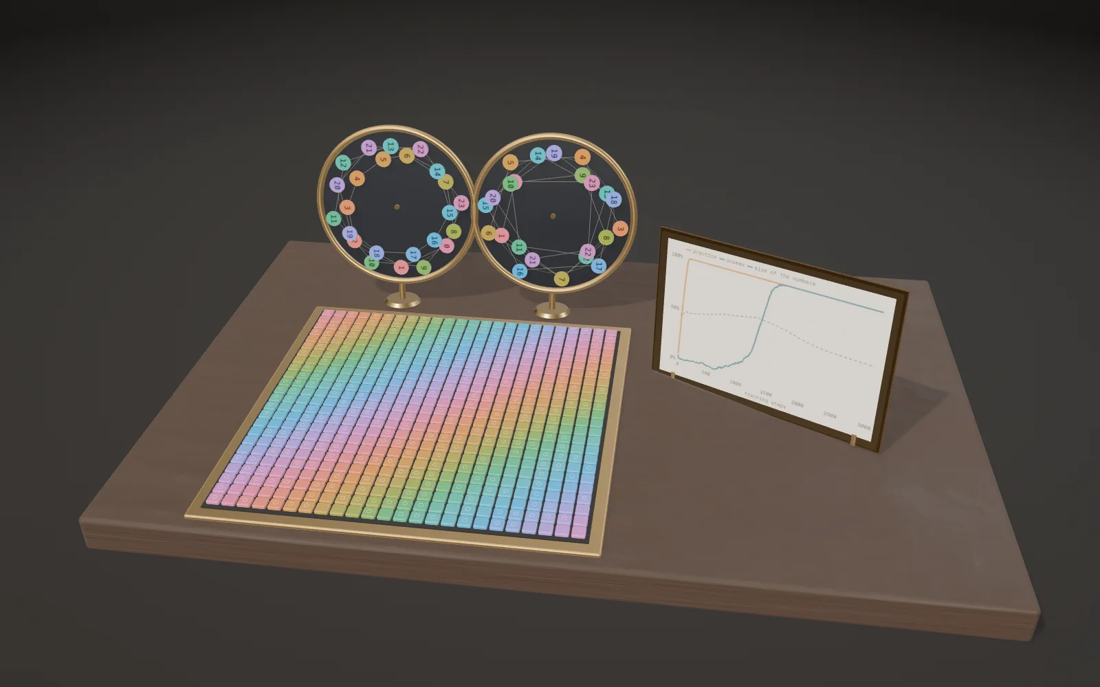 Plate 46Learning by Heart, Then Learning the RuleA small neural network learns to add hours on a 24-hour clock. It gets its practice questions right almost at once, by memorising them, and only long afterwards answers questions it has never seen. Inside, it has built clocks.