The Bell Test
Two entangled photons fly apart to two analysers, each set at random. The correlation they count passes the most any theory of answers fixed in advance allows. The 2022 Nobel Prize in Physics went to the three who showed it.
Scroll
Past Two
A Bell test boils its results down to one number, S. If the world is “locally real”, meaning each particle carries its answers with it and nothing done far away can affect it here, S can never be larger than 2 (or smaller than −2). Quantum mechanics predicts it can reach 2√2, about 2.83.
In 1982 Alain Aspect’s group at Orsay, France, measured S = 2.697 ± 0.015, where quantum mechanics predicted 2.70 ± 0.05 for their apparatus. In 1998, with two stations 400 m apart in Innsbruck, an experiment measured S = 2.73 ± 0.02, 30 standard deviations beyond 2.
Local models |S| ≤ 2 · quantum mechanics 2√2 ≈ 2.83 · 1982: 2.697 ± 0.015
1.3 Kilometres
In 2015 an experiment in Delft, the Netherlands, placed two electron spins 1.3 km apart, each held in a defect of a diamond (an NV centre). Light takes 4.27 µs to cross between them; choosing each measurement at random and reading out the result were both done within that time, too soon for any signal at the speed of light to reach the other side.
Every trial gave a result, so none could be picked out. Over 245 trials it found S = 2.42 ± 0.20; the chance that a local model would show a violation this large is at most 3.9 %. It was the first test to close the locality and detection loopholes at once. The same year, groups in Vienna and at NIST in the United States did the same with photons and efficient detectors, with far stronger statistics.
1,280 m · light takes 4.27 µs · 245 trials · S = 2.42 ± 0.20 (Delft, 2015)
Photons in Pairs
A pair of entangled photons leaves the same crystal, one to each analysis station. Each analyser can be turned to any angle; a photon comes out either at its “+” port or at its “−” port.
Seen from one side alone, the results are completely random, half and half, however the other side is turned. Only when the two records are compared does a pattern appear: with both analysers at the same angle, the results always agree; at an angle θ apart, they agree a fraction cos²θ of the time; 90° apart, they always differ.
Fraction alike = cos²(a − b) · one side alone: 50 % each
The CHSH Sum
In 1964 John Bell proved that any local hidden-variable theory puts a limit on such correlations. In 1969 Clauser, Horne, Shimony and Holt wrote it in a form experiments can test: each side has two angles, a and a′, b and b′; measure the correlation E for all four pairings and add them up as S = E(a,b) − E(a,b′) + E(a′,b) + E(a′,b′).
If every pair carried its answers in advance (+1 or −1 for each angle), then however they were chosen, each pair would give exactly +2 or −2, so the average can never pass 2. At the angles 0°, 45° and 22.5°, 67.5°, quantum mechanics gives 2√2. In 1980 Boris Tsirelson proved that quantum mechanics can never go higher.
S = E(a,b) − E(a,b′) + E(a′,b) + E(a′,b′) · a 0°, a′ 45°, b 22.5°, b′ 67.5°
Best Local Model
Could answers carried in advance imitate quantum mechanics? A simple model: each pair sets off sharing one random “hidden polarisation”, and each analyser looks only at that and its own angle, sending the photon out of whichever port is closer to it.
Seen from one side, this model is half and half too; with the analysers at the same angle or 90° apart, it agrees with quantum mechanics. In between it differs: its correlation falls in a straight line with the angle, where quantum mechanics follows a cosine. At the CHSH angles it gives exactly 2, as far as any local model can go; quantum mechanics gives 2.83.
Local: E = 1 − 4θ/180° · quantum: E = cos 2θ · both counted pair by pair by this page
Cut Open
At the back of the table is a 405 nm violet laser; a mirror and a lens focus its light into a BBO crystal. After the crystal come two compensating crystals, then two small mirrors that pick the photon pairs off either side of the violet beam and send them into fibre; the violet light that is left ends in a beam dump.
The fibre runs through two reels to two stations, left and right. Each station has, in turn, a collimator, a Pockels cell, a half-wave plate in a motorised rotation mount, a polarising beam-splitter cube, and two single-photon detectors, “+” and “−”. Four cables lead to the coincidence counter at the front. The stations’ light path is cut open.
Station A on the left, B on the right · one table is schematic: in experiments they stand metres to over a kilometre apart
One Becomes Two
Some crystals respond to light in a way that is not linear. In a crystal of BBO (beta barium borate), now and then one 405 nm violet photon splits into two 810 nm infrared ones, keeping both energy and momentum. This is spontaneous parametric down-conversion. Nearly all the violet photons simply pass through.
In type-II down-conversion the two photons leave along two cones, the light on one polarised horizontally, on the other vertically. The cones cross at two places, left and right. A pair leaving there cannot be said to be horizontal and vertical either way round, only opposite: that is entanglement. In 1995 Kwiat, Zeilinger and colleagues in Innsbruck used such a source to get more than 1,500 pairs a second.
405 nm → 810 + 810 nm · the two crossings are about 6° apart in reality, drawn wider
Random Settings
Turn a half-wave plate by θ and the light’s polarisation turns by 2θ; the polarising beam-splitter cube after it lets one polarisation through and reflects the one at right angles. So the analyser’s angle is twice the wave plate’s.
To rule out the two sides being in league, each angle must be set while the photons are in flight, and set at random. In 1982 Aspect’s group used acousto-optic switches flipping between two directions about every 10 ns; the switches were 12 m apart, 40 ns for light. But the switching was quasi-periodic, not truly random. The 1998 Innsbruck experiment used physical random-number generators and electro-optic modulators.
Wave plate θ → polarisation 2θ · 1982: switching every 10 ns, 12 m · 1998: 400 m, random numbers
Counting Pairs
Behind each port is a single-photon detector: one photon in, one electrical pulse out. The coincidence counter stamps each pulse with its time and treats pulses on the two sides within a few nanoseconds as one pair, counted as ++, +−, −+ or −−. The correlation is E = (N++ + N−− − N+− − N−+) / N.
Photons the detectors miss leave a loophole: if only some are recorded, a local model could choose which. A maximally entangled state needs an overall efficiency above 82.8 %; Eberhard showed in 1993 that with less entangled states the threshold falls, towards a limit of two-thirds. In 2001 an experiment with trapped ions closed this loophole first. In 2015 Vienna’s transition-edge sensors reached overall efficiencies of about 78.6 % and 76.2 %, and NIST’s superconducting nanowires about 75 %.
E = (N₊₊ + N₋₋ − N₊₋ − N₋₊) / N · threshold 82.8 %, limit 2⁄3
Fifty Years
In 1972 Stuart Freedman and John Clauser ran the first such test with pairs of photons from calcium atoms. After about 200 hours of counting, the result broke the inequality of local realism and agreed with quantum mechanics. In 1982 Aspect’s experiments measured more precisely and, for the first time, switched the angles while the photons were in flight.
Anton Zeilinger’s group used entanglement to do new things: quantum teleportation in 1997, carrying one photon’s polarisation state over to another photon, and entanglement swapping in 1998, which entangled two photons that had never met. The 2022 Nobel Prize in Physics was shared equally by Aspect, Clauser and Zeilinger, “for experiments with entangled photons, establishing the violation of Bell inequalities and pioneering quantum information science”. How qubits are built is the plate “Superconducting Qubits and Error Correction”.
1964 Bell · 1972 · 1982 · 1997–98 · 2015 · 2022 Nobel Prize
Taken Apart
The pump laser, the optics, the BBO crystal, the couplers, the fibre reels, and at each station the Pockels cell, wave plate, cube, detectors and random-number generator, then the coincidence counter, come apart piece by piece.
Whichever piece the pointer rests on is lifted out and the rest fade; left alone, the pieces are all named.
Two Angles
The two levers are the angles a and b at stations A and B; each station’s second angle is its first plus 45°. As each pair arrives, each side tosses a coin to choose which of its angles to use. The upper row samples quantum mechanics; the lower row samples the best local model, pair by pair, at the same angles.
With b 22.5° past a, the quantum S is largest, 2√2, and the local model gives exactly 2. The error bars shrink as more pairs are counted: about ±0.03 after ten thousand.
Try thisTurn station B from the same angle as A to 45° past it: where is the quantum S largest, and what does the best local model give there?
What the model leaves out
The table follows the layout that photon Bell tests share in their published descriptions: a pump laser, a nonlinear crystal, fibre, fast switches at two stations, polarisation analysers, single-photon detectors and a coincidence counter. Sizes are common ones; the arrangement is schematic, not any laboratory’s plans. In experiments the stations stand metres to over a kilometre apart; here they share one table, and the fibre reels stand for the distance between them. The cones and the angle between the two photons’ paths are drawn about three times wider. Photons are drawn as visible beads, about a billion times slower than light; 810 nm light is invisible to the eye. The detectors are drawn as common avalanche-diode modules; the loophole-free tests of 2015 used superconducting detectors in cryostats, and crystals of periodically poled KTP rather than BBO. The laboratory samples ideal pairs: no noise, every photon detected, no accidental coincidences in the time window.
Some common misreadings
A violation of Bell’s inequality means two things cannot both hold: that results are fixed before they are measured (realism), and that a choice made far away cannot affect them here (locality). It cannot send messages faster than light: seen from one side, the results are always half and half and show nothing of the other side’s angle; the correlation appears only when the two records are brought together, and carrying the records takes an ordinary signal. A “loophole” is a local explanation an experiment has not ruled out, not a flaw in the theory. What remains after 2015 is the assumption of “freedom of choice”: that the random numbers picking the angles have nothing to do with the photons. In 2017 one experiment picked its angles with starlight from the Milky Way emitted some 600 years earlier; in 2018 the “BIG Bell Test” used key presses from about 100,000 volunteers. The superposition here is that of quantum states; the phenomenon of the same name in neural networks is the plate “More Features Than Neurons”.
Common questions · 4
- How large can S get in a Bell test?
If the world is “locally real”, meaning each particle carries its answers with it and nothing done far away can affect it here, S can never be larger than 2 (or smaller than −2). Quantum mechanics predicts it can reach 2√2, about 2.83.
01Past Two ↑- How was the first loophole-free Bell test done?
In 2015 an experiment in Delft, the Netherlands, placed two electron spins 1.3 km apart, each held in a defect of a diamond (an NV centre).
021.3 Kilometres ↑- How are entangled photons made?
In a crystal of BBO (beta barium borate), now and then one 405 nm violet photon splits into two 810 nm infrared ones, keeping both energy and momentum.
07One Becomes Two ↑- Who won the 2022 Nobel Prize in Physics?
The 2022 Nobel Prize in Physics was shared equally by Aspect, Clauser and Zeilinger, “for experiments with entangled photons, establishing the violation of Bell inequalities and pioneering quantum information science”.
10Fifty Years ↑
Sources
- Nobel Prize: press release for the 2022 Physics prize (Alain Aspect, John F. Clauser, Anton Zeilinger, shared equally)
- Nobel Committee for Physics: scientific background to the 2022 prize
- J. S. Bell (1964): On the Einstein Podolsky Rosen paradox, Physics 1, 195
- J. F. Clauser, M. A. Horne, A. Shimony, R. A. Holt (1969): PRL 23, 880 (the CHSH inequality)
- S. J. Freedman, J. F. Clauser (1972): PRL 28, 938 (calcium cascade; δ = 0.050 ± 0.008; about 200 h)
- B. S. Cirel’son (1980): Quantum generalizations of Bell’s inequality, Lett. Math. Phys. 4, 93 (2√2)
- A. Aspect, P. Grangier, G. Roger (1982): PRL 49, 91 (S = 2.697 ± 0.015; quantum prediction 2.70 ± 0.05)
- A. Aspect, J. Dalibard, G. Roger (1982): PRL 49, 1804 (acousto-optic switches near 50 MHz, about every 10 ns; 12 m, 40 ns; quasi-periodic)
- P. H. Eberhard (1993): Phys. Rev. A 47, R747 (the efficiency threshold)
- P. G. Kwiat et al. (1995): PRL 75, 4337 (a type-II BBO source; two crossing cones; over 1,500 pairs a second)
- D. Bouwmeester et al. (1997): Experimental quantum teleportation, Nature 390, 575
- J.-W. Pan, D. Bouwmeester, H. Weinfurter, A. Zeilinger (1998): Experimental entanglement swapping, PRL 80, 3891
- G. Weihs et al. (1998): PRL 81, 5039 (400 m apart; random-number generators and electro-optic modulators; S = 2.73 ± 0.02, 30 standard deviations)
- M. A. Rowe et al. (2001): Nature 409, 791 (trapped ions; 2.25 ± 0.03; the detection loophole closed)
- B. Hensen et al. (2015): Nature 526, 682 (Delft; 1.3 km; 245 trials; S = 2.42 ± 0.20; P ≤ 0.039)
- M. Giustina et al. (2015): PRL 115, 250401 (Vienna; transition-edge sensors; 78.6 % / 76.2 %; 3.74 × 10⁻³¹)
- L. K. Shalm et al. (2015): PRL 115, 250402 (NIST; superconducting nanowire detectors; 74.7 % / 75.6 %)
- J. Handsteiner et al. (2017): Cosmic Bell test, PRL 118, 060401 (Milky Way stars; about 600 years)
- The BIG Bell Test Collaboration (2018): Nature 557, 212 (about 100,000 participants)
- A. Aspect: Bell’s theorem: the naive view of an experimentalist, arXiv:quant-ph/0402001 (no faster-than-light telegraphy)
- N. Brunner et al. (2014): Bell nonlocality, Rev. Mod. Phys. 86, 419 (82.8 % and 2⁄3)
Data
The optical table follows the layout that photon Bell tests share in their published descriptions (a pump laser, a nonlinear crystal, fibre to two stations with fast setting switches, polarising analysers, single-photon detectors and a coincidence counter); it is not drawn from any one laboratory’s plans. The counts, correlations and S values in the figures and the laboratory are computed by this page; they are not measured data. Material presets, parts and the softbox studio of the site’s model kit are ported from AirsupHQ/machine-skill (MIT, © 2026 Air Supply Technologies Inc.).
The text, pictures and models on this page are licensed CC BY-NC 4.0: free to use and adapt for teaching and other non-commercial purposes, with credit to world.lapla.si. Third-party material listed above keeps its own licence.
Cite this plate
Laplace’s Mini World, Plate F24, “The Bell Test”, https://world.lapla.si/en/bell/, CC BY-NC 4.0, updated 2026-10-20.
Follow the question
 Plate F17Superconducting Qubits and Error CorrectionA chip the size of a fingernail holds 97 superconducting circuits. Each one makes mistakes; together they make a “logical qubit” that gets more reliable as it grows.
 Plate 43More Features Than NeuronsA single neuron in a neural network often stands for several unrelated things. A model with just two neurons can arrange five features into a pentagon and keep them all.