How a Neural Network Learns
A neural network learns by doing one thing again and again: measure how wrong it is, work out which way and how far to turn every one of its numbers, and turn them a little. Working out how to turn every number at once is called backpropagation. The network on this bench is training in your browser: the relief is its real error, and every step of the steel ball is a real gradient.
Scroll
Learning Is Turning Numbers
At the back of the bench is a small neural network. On the left, two inputs: the two coordinates of a point. In the middle, two layers of 6 units. On the right, one output: how sure it is that the point is red. Each glass rod carries a number, its weight, and each unit has a bias. 67 numbers in all.
The tile in front holds 160 points in two spirals. At first the numbers are random and the network gets almost everything wrong. Training repeats one thing: show it a few points, measure how wrong it is (the loss), and turn all 67 numbers a little so the loss goes down. The gauge on the right shows the loss; the tile’s shading is what the network thinks now.
2 → 6 → 6 → 1 · 67 numbers · training live on this page
The Shape of the Error
Hold 65 of the 67 numbers still and leave two rods free to turn, the two with red bands. Every setting of the two gives a loss. Spread all the settings over a plane, make the height the loss, and you have this terrain. The aluminium block is milled to the loss this network really computes.
The ball sits where the two weights are now; the sliders at the front and the left read them. Its height is the loss now. Learning means getting the ball downhill.
Across and along: the two weights · height: the loss (log scale) · a contour every quarter of a power of ten
The Steepest Way Down
The ball cannot see the terrain, only feel the slope under it. At every point the direction that climbs most steeply is the gradient. The brass needle points the other way, the steepest way down; the longer the needle, the steeper the slope.
Gradient descent is: take a small step along the needle, feel the slope again, step again. Cauchy wrote the method down in 1847, to solve systems of equations.
Each step: weights ← weights − learning rate × gradient
How Big a Step
How far each step goes is the learning rate, the knob at front left. Too small, and after dozens of steps the ball is still on the hillside. About right, and it is down in the valley in a dozen or so. Too big, and the first step overshoots the valley and up the far slope, and the ball works its way back. A little bigger, and it is thrown straight off the terrain.
For a bowl-shaped valley the limit can be worked out: a learning rate above 2 divided by the curvature of the steepest direction always diverges. A real network’s terrain changes from place to place, and the limit has to be found by trying.
Learning rate: 0.1 too small · 1.5 about right · 4.2 too big · 6 thrown off
A Handful of Data
An exact gradient needs all 160 points. Large models train on hundreds of billions of tokens; reading them all for every step is impossible. Instead, each step takes a small random handful, say 16 points, and uses their gradient for the whole.
That direction is noisy: the thin steel needle is the gradient of all the data, the brass needle that of this handful, and they never quite agree. The ball wanders, but on average it goes down. This is stochastic gradient descent; its mathematics begins with Robbins and Monro’s stochastic approximation of 1951.
16 points a step · the points lit on the tile are this step’s
Momentum and Adam
This terrain has a long, flat valley floor: a steep wall on one side, and almost no slope along the floor. Plain gradient descent (the steel ball) drops in, and then each step is shorter than the last. On other terrain it would also zigzag between the walls.
Give the ball momentum (the brass ball): each step keeps nine tenths of the last step’s velocity, and the faint slope along the floor builds up into speed. Adam (the blued ball) does it another way: it scales each weight’s step by the size of its own gradients, small where it is steep, larger where it is flat. All three start from the same point and take 140 steps. Large models today are mostly trained with methods of the Adam family.
Steel: gradient descent (rate 2) · brass: momentum 0.9 (0.3) · blued: Adam (0.2)
Forward: Compute It Once
To know which way the ground slopes, first compute the loss. Take a point on the tile; its two coordinates enter the network on the left. Each unit multiplies what comes in by the weights on its rods, adds them up, passes the sum through an S-shaped function (tanh) and hands it to the next layer. The amber light is those numbers travelling right.
Each unit, once done, keeps its value in the vial beside it. The last unit gives how sure the network is that the point is red; compared with the right answer, that is the loss for this point.
Each unit: z = Σ weight × input + bias, value = tanh(z) · every value is kept
Backpropagation
Now: how should each of the 67 numbers turn? The chain rule says the loss’s rate of change with a rod is “the loss’s rate of change with the unit at the rod’s output end” times “the value of the unit at its input end”. The first travels back from the output, layer by layer (the blue light); the second was kept in the vials on the way forward.
So one pass from output to input gives every rod its share: how much of this error each rod is responsible for, all at once. In 1986 Rumelhart, Hinton and Williams used it in Nature to train networks with hidden layers, and it became widely known; the same backward method had been written down by Linnainmaa in 1970, to estimate rounding errors.
The error signal δ runs back from the output · each rod’s gradient = δ at its output end × the value kept at its input end
What the Backward Pass Costs
A gradient can be had without backpropagation: turn one rod a tiny bit and see how the loss changes. But every number needs its own trial, nudged up and nudged down: for this network’s 67 numbers, 134 more passes.
One backward pass costs about two forward passes in multiply-adds, however many numbers there are. Here each point takes 54 multiply-adds forward and 96 backward; trying them one by one takes 7,236. GPT-3 has 175 billion numbers: trying them one by one would take 350 billion passes for a single step; backpropagation takes about three passes’ worth.
Multiply-adds per point: forward 54 · backward 96 · one by one 7,236
Fading on the Way Back
Make the network deep and trouble starts. Each layer the error signal travels back, it is multiplied by a layer of weights and by a slope. The S-shaped sigmoid’s slope is at most 1/4; after seven layers the first layer’s gradient is about a ten-thousandth of the last one’s, and the early rods barely learn. These are vanishing gradients. With weights too large, the same products grow instead: exploding gradients.
The fixes came one at a time: scaling the starting weights by each layer’s width (Glorot and Bengio, 2010), functions whose slope does not keep shrinking (tanh, ReLU), and later residual connections and normalisation.
Seven layers, the same points: the gradient’s size in each layer with sigmoid and with tanh
Why It Scales
The cost of backpropagation does not get worse as the network grows: a step is always about three forward passes. A network a thousand times larger costs a thousand times more per step, not a million.
GPT-3’s 175 billion numbers were trained on 300 billion tokens, about 3.14 × 10²³ floating-point operations in all: 6 per number per token, 2 forward and 4 backward. Every update was one forward pass, one backward pass and a small step downhill, as on this bench with 67 numbers.
Per parameter, per token: 2 forward + 4 backward = 6 floating-point operations
The Bench
Choose a data set or place your own points on the tile; set the learning rate, the points per step, momentum or Adam, the width and depth of the network; step, or let it run. The relief is the loss over the two rods: the other numbers are moving, so the terrain moves too.
Try thisTurn the learning rate above 3 and press Run. Where does the ball go? Switch to Adam at the same rate.
What the model leaves out
The network on the bench is tiny: two inputs, two layers of 6 units, 67 numbers, 160 points. The relief is one slice: the real loss is a surface in 67 dimensions; here the other 65 numbers are held still (on the bench they move) and only two rods vary. The height is milled to the logarithm of the loss, which flattens the deepest valleys somewhat. In the early chapters the ball moves only in these two dimensions, by those two rods’ real gradient. Real large models have billions to trillions of numbers, change their learning rate as they train, and are computed on many GPUs at once. The light in the glass rods is an illustration: its brightness is the size of the signal or the gradient the rod carries now.
Common misunderstandings
Gradient descent does not promise the lowest point. It only promises a little downhill at each step: it can stop on a plateau, drop into a local hollow, or creep along a valley. In large networks this is often not so bad, since many different low places are equally good. Nor is backpropagation the learning itself: it only computes the gradient; which way to go and how far is the optimiser’s business. Whether the brain learns this way is not settled.
Common questions · 4
- How big can the learning rate be?
For a bowl-shaped valley the limit can be worked out: a learning rate above 2 divided by the curvature of the steepest direction always diverges.
04How Big a Step ↑- Who came up with backpropagation?
In 1986 Rumelhart, Hinton and Williams used it in Nature to train networks with hidden layers, and it became widely known; the same backward method had been written down by Linnainmaa in 1970, to estimate rounding errors.
08Backpropagation ↑- What are vanishing gradients?
The S-shaped sigmoid’s slope is at most 1/4; after seven layers the first layer’s gradient is about a ten-thousandth of the last one’s, and the early rods barely learn.
10Fading on the Way Back ↑- How much computing did GPT-3 take to train?
GPT-3’s 175 billion numbers were trained on 300 billion tokens, about 3.14 × 10²³ floating-point operations in all: 6 per number per token, 2 forward and 4 backward.
11Why It Scales ↑
Sources
- Rumelhart, Hinton & Williams (1986): Learning representations by back-propagating errors, Nature 323:533–536
- Linnainmaa (1976): Taylor expansion of the accumulated rounding error, BIT 16:146–160 (the reverse method of his 1970 master’s thesis)
- Griewank (2012): Who Invented the Reverse Mode of Differentiation?, Documenta Mathematica (history; the cost of a gradient)
- Werbos (1982): Applications of advances in nonlinear sensitivity analysis (his 1974 thesis’s method applied to neural networks)
- Lemaréchal (2012): Cauchy and the gradient method (Cauchy, 1847)
- Robbins & Monro (1951): A Stochastic Approximation Method, Ann. Math. Statist. 22:400–407
- Polyak (1964): Some methods of speeding up the convergence of iteration methods (momentum)
- Kingma & Ba (2014): Adam: A Method for Stochastic Optimization, arXiv:1412.6980
- LeCun, Bottou, Orr & Müller (1998): Efficient BackProp (the limit 2/λmax; stochastic learning)
- Hochreiter (1991): Untersuchungen zu dynamischen neuronalen Netzen (vanishing gradients)
- Bengio, Simard & Frasconi (1994): Learning long-term dependencies with gradient descent is difficult
- Glorot & Bengio (2010): Understanding the difficulty of training deep feedforward neural networks
- He et al. (2015): Delving Deep into Rectifiers, arXiv:1502.01852
- Brown et al. (2020): Language Models are Few-Shot Learners, arXiv:2005.14165 (GPT-3, Table D.1)
- Kaplan et al. (2020): Scaling Laws for Neural Language Models, arXiv:2001.08361 (about 6 operations per parameter per token)
- Li et al. (2018): Visualizing the Loss Landscape of Neural Nets, arXiv:1712.09913
Data
The network, its training and the relief are the site’s own: a small multilayer perceptron trained in your browser by src/topics/backprop/nn.js, with hand-written backpropagation; the relief is the loss it computes over two of its weights.
The text, pictures and models on this page are licensed CC BY-NC 4.0: free to use and adapt for teaching and other non-commercial purposes, with credit to world.lapla.si. Third-party material listed above keeps its own licence.
Cite this plate
Laplace’s Mini World, Plate F17, “How a Neural Network Learns”, https://world.lapla.si/en/backprop/, CC BY-NC 4.0, updated 2026-10-17.
Watch next
The player comes from YouTube and loads only when you press play.
Follow the question
 Plate F13Attention in TransformersA two-layer, eight-head Transformer reads a sentence in your browser, one character at a time, and guesses the next. Each thread is one act of attention; its brightness is the weight.
 Plate 44Pictures Out of NoiseMany AI image generators start from random static and remove it, one step at a time. A small network does the same in your browser, and a cloud of dots slowly condenses into a knot.
 Plate 46Learning by Heart, Then Learning the RuleA small neural network learns to add hours on a 24-hour clock. It gets its practice questions right almost at once, by memorising them, and only long afterwards answers questions it has never seen. Inside, it has built clocks.
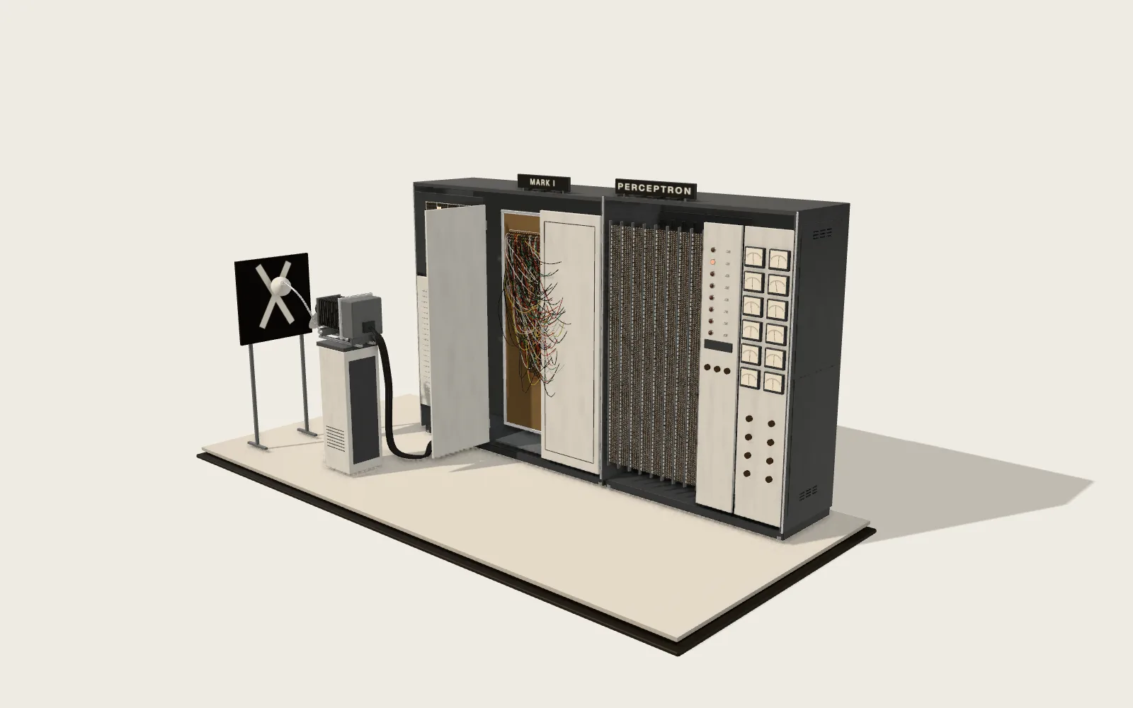 Plate C15The Mark I PerceptronA machine that learned letters from examples: four hundred photocells to see, 512 randomly wired units in between, and motor-driven potentiometers to remember.